A transformer guided multi modal learning framework for predictive and causal assessment of thermal runaway in high energy batteries

This section discusses the Integrated Transformer-Guided Multi-Modal Learning Framework for Predictive and Causal Assessment of Thermal Runaway in High-Energy Batteries, highlighting its inefficiencies and inherent complexity. Figure 2 illustrates the model architecture of the proposed analysis process, while Fig. 3 depicts the overall flow of the proposed analysis process.

Framework principles and architecture

The ST-Former operates on time-sequenced thermal image frames T{x, y,t} ∈ R’{H×W×T}, in which, for this procedure, H, W, and T are referred to as image height, width, and temporal depth respectively. Each thermal frame is first partitioned into fixed-size patches p{i, j,t} and embedded using a linear projection ‘E’ in process. The output is the initial token sequence zt’{(0)} ∈ R’{N×d}, where N is the number of patches and ‘d’ the embedding dimension sets. A spatiotemporal positional encoding P(x, y,t) is then added to encode location and time-dependent priors via Eq. 1.

ST-Former integrates complementary but independent modality sources. High-resolution infrared cameras capture thermal images to generate frame-based temperature fields, T(x, y,t), with a resolution of 640 × 480 pixels and a temporal sampling rate of 50 Hz. These thermal images are pre-processed into non-overlapping 16 × 16 patches, which are linearly projected into latent vectors to preserve fine-grained heat-gradient variations. Thermal imaging alone cannot capture electrochemical states or cell dynamics. To address this, synchronized voltage, current, and ambient temperature signals are recorded at 1 Hz. Together, these heterogeneous modalities form the multimodal priors used in ST-Former.

The model enhances temporal self-attention by jointly encoding thermal patches and sensor logs. Spatial temperature patches highlight localized thermal hotspots across time, while sensor measurements capture electrochemical and thermal dynamics. The two embeddings are concatenated prior to token-level positional encoding, enabling the model to temporally link localized temperature rises with changes in current or voltage. Through this design, ST-Former predicts thermal instability events by jointly leveraging localized thermal-gradient intensifications and global operating conditions. Experimental evaluation shows that incorporating sensor logs improves predictive performance, increasing AUC-ROC by 3.5% compared to a thermal-only baseline.

Fig. 2

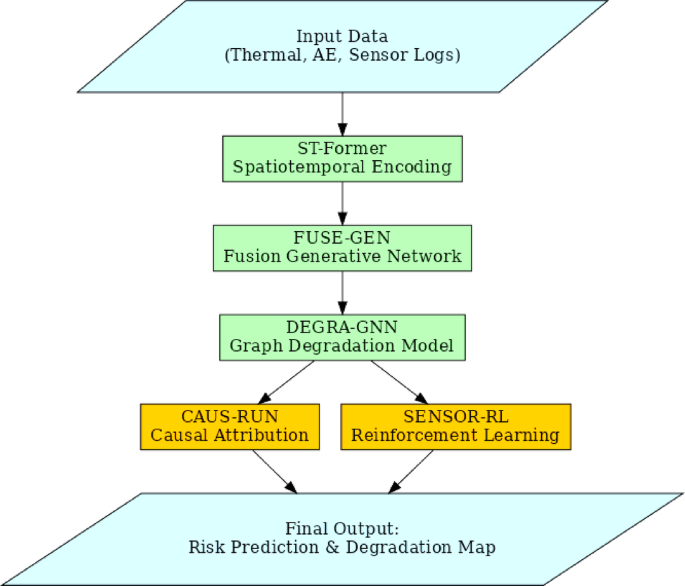
Model Architecture of the Propsoed Analysis Process.

The self-attention mechanism is then applied over the token sequence to capture long-range dependencies, modeled via Eqs. 2–5.

where, WQ, WK, WV ∈ R‘{d×dk} are learnable matrices for this process. The resulting contextually enriched embedding Rt ∈ R‘{512} serves as the initial risk representation, updated per second to reflect dynamic thermal changes. Iteratively, Next, as per Fig. 3, The risk embeddings Rt are subsequently fused with frequency-domain representations of AE signals through the FUSE-GEN modules. The AE signals At ∈ R’f, processed using short-time Fourier transform over the 20 kHz band, yield latent vectors z{AE} in the process. The thermal embeddings Rt are simultaneously projected to latent thermal vectors z{TH} in the process. Both modalities are encoded via individual encoders E{AE} and E{TH} and fused using a shared latent space in a Variational Autoencoder (VAE) formulation via Eqs. 6 & 7.

The joint latent representation Jt ∈ R‘{1024} is derived from the fused encoding, where the KL-divergence regularization enforces tight coupling between AE and thermal modalities to preserve their shared degradation semantics. The fused latent vector Jt is passed to DEGRA-GNN for electrode-level degradation tracking sets. The battery cell is modeled as a graph G = (V, E), where each node vi ∈ V represents an electrode segment and edges e{ij} ∈ E represent thermal and electrical interaction pathways. Each node vi is initialized with features hi’0 = φ (Jt, γi), where γi encodes static spatial position. A Graph Attention Network (GAT) updates node features iteratively via Eqs. 8–10.

Fig. 3

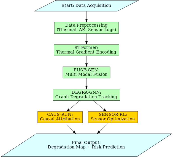
Overall Flow of the Proposed Analysis Process.

These updates are applied over ‘T’ timestamp steps to model the evolution of degradation sets. Via Eq. 11, residual energy per node defines the degradation function as an integral over energy residuals.

where, κ{ij} represents the thermal conductivity between nodes i and j, while Ti(τ) is the temperature of node ‘i’ at timestamp ‘τ’ sets. The spatial degradation map D{i, j,t} builds up applying interpolation of the node-wise degradation scores over the 2D electrode topology using bilinear surface fitting via Eq. 12.

where, ψk(i, j) are spatial interpolation weights derived from proximity functions. The final risk propagation equation for the cell structure aggregates time-evolved nodal risks modified by the latent fusion and thermal-attentive weights via Eqs. 13, 14

This differential risk projection provides the real-time degradation distribution over the battery surface and serves as the final predictive output of the pipelines.

Figure 4 illustrates the Data Flow of the Proposed Analytical Process. The Spatiotemporal Transformer for Thermal Gradient Encoding (ST-Former), Multi-Modal Generative Fusion Network for AE-Thermal Co-Learning (FUSE-GEN), and Graph-Based Electrode Thermal Degradation Tracker (DEGRA-GNN) built in the proposed framework is motivated to create a framework having hierarchical structure capable of extracting, fusing, and projecting complex risk signals from multi-modal battery data streams. Recent graph neural network investigations in system dependability and safety have focused on mission-critical measurements and interpretability57. Inspired by recent achievements, DEGRA-GNN models electrode-level fault propagation using graph-based learning for structural accuracy and causal insights. The architecture develops the pipeline with information flowing continuously from fine-grained thermal feature encoding to latent multi-modal signal integration and ends up with graph-based spatiotemporal degradation modeling. The pipeline integrates global and local contexts of degradation phenomena using physics-informed battery dynamics and deep learning. Transformer-based perception, multi-modal generative fusion, and graph-guided degradation modeling form closed analytical loops. Each stage complements the next by localizing degradation risks from high-dimensional perceptual data. Both macro- and micro-level deterioration cues are jointly learned and interpreted.

Interpretability and optimization modules

To enhance forward-looking battery risk prediction, we designed two modules: CAUS-RUN (Counterfactual Thermal Runaway Attribution) and SENSOR-RL (Sensor Prioritization via Reinforcement Learning), which improve interpretability and operational efficacy. While ST-Former, FUSE-GEN, and DEGRA-GNN encode, fuse, and propagate degradation patterns across spatial and temporal domains, their outputs remain black-box in nature. To address this limitation, CAUS-RUN provides causality-aware interventions, attributing thermal risk zones to decision-relevant variables.

Fig. 4

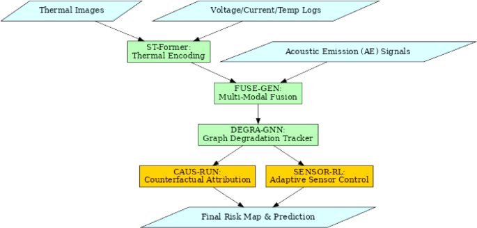
Data Flow of the Proposed Analysis Process.

Using real-time battery data, SENSOR-RL dynamically optimises sensor operation to maintain energy and computational restrictions. In a diffusion-based generative framework, CAUS-RUN models thermal evolution counterfactually using SCM. For a given observed thermal sequence T{x, y,t} and an associated degradation map D{i, j,t}, the diffusion generator G{θ} is trained to yield such perturbed thermal trajectories T̃{x, y,t}‘{δ} that the Identity Represented Via Eq. 15 is fulfilled in this,

where, δ{x, y,t} ∼ N(0,σ²) represents controlled perturbations injected into temperature trajectories. The goal is to evaluate whether a specific perturbation results in significant risk change via Eq. 16,

where, MR is the risk inference model, such as DEGRA-GNN or FUSE-GEN in process. A counterfactual attribution indicator is defined via Eq. 17,

This binary mask highlights spatial zones where thermal perturbations yield significant deviations in risk estimates satisfying a predefined threshold \(\epsilon\) sets. To further restrict attribution to causal interactions, an SCM S is defined over the observed variables X = {T, A, V, I}, modeled via structural equations represented via Eq. 18.

where, Pa(Xi) represents the parent variables in the causal graph, and Ui are exogenous noise terms. The causal effect of intervention do (T{i, j,t} = t′) on risk is evaluated via Eq. 19,

A region is considered causally contributory if this expectation exceeds a significance threshold τ, producing the final causal attribution map C{i, j,t} in process. By incorporating these attribution scores into the learning process, upstream modules can also be regularized by applying an auxiliary causal loss Via Eq. 20,

Complementing this interpretability module, SENSOR-RL introduces an interactive sensing policy capable of online adaptation to minimize energy consumption without sacrificing risk-prediction-quality sets. The sensor control policy is represented by π(at | st), where the action at corresponds to sensing parameters (e.g., imaging frequency, AE trigger thresholds), and state st consists of risk embeddings Rt, system health logs (SoC, State-of-Charge; SoH, State-of-Health), and confidence margins ηt in process. A reward function R(st, at) is defined via Eq. 21,

where the accuracy is derived from ROC-AUC or degradation localization scores, and energy is estimated via Eq. 22,

With, ‘ck’ stands for cost per sensor and δk(at) for sensor usage under action ‘at’ sets. The policy π is optimized with the use of Proximal Policy Optimization (PPO), with the objective function J(θ) defined via Eqs. 23, and 24,

And Ât as the advantage estimate from Generalized Advantage Estimation (GAE) via Eq. 25,

where each temporal difference δt is given via Eq. 26,

This design allows SENSOR-RL to learn optimal sensing schedules that are at the same time context-dependent, risk-aware, and cost-sensitive in process. The output of the entire system is a degradation prediction map D̂{i, j,t}, optimized by adaptive sensor control πt, dynamically validated within the causal attribution au via maps C{i, j,t} for this process. Thus, the entire pipeline predicts imminent thermal runaway events and explains the source of risk with a sensory footprint that adapts for real-time feasibility via Eqs. 27, and 28,

This method enables SENSOR-RL to learn context-dependent, risk-aware, and cost-sensitive sensing schedules. The framework generates a degradation prediction map D̂{i, j,t}, optimized through adaptive sensor control πt, and dynamically validated via causal attribution maps C{i, j,t}. The sensory footprint defined in Eqs. (27) and (28) adapts in real time to ensure feasibility, thereby supporting both thermal runaway event prediction and pipeline risk interpretation.

For battery safety evaluation, the final equation integrates prediction, interpretability, and computational efficiency to enable causally relevant, sensor-adaptive, graph-based degradation forecasting. Next, we discuss efficiency of the proposed model by different metrics and compare it with existing models in various scenarios.