

The proposed control framework is developed to achieve four key objectives that ensure the efficient and stable operation of the microgrid. These objectives focus on optimizing power extraction from renewable energy sources, regulating the battery’s charging and discharging processes, and maintaining grid stability with high power quality:
-
(i)
Maximum/Adaptive Power Point Tracking (MPPT/APPT): The voltages of the photovoltaic system (\(V_{pv}\)) and the wind turbine (\(V_{w}\)) must accurately follow their respective optimal reference values (\(V_{pvopt}\) and \(V_{wopt}\)). These reference values are dynamically determined by two optimizers, thereby ensuring that both systems continuously operate at their optimal power point.
-
(ii)
Power Factor Correction (PFC): The grid current (\(i_g\)) must be sinusoidal, matching the frequency and phase of the grid voltage (\(V_g\)). The last two control objectives depend on the battery’s state of charge (SOC):
-
(iii)
Constant Current (CC) Mode: During this stage, the battery current \(i_b\) is regulated to follow a constant reference value \(i^*_{b}\), which represents the maximum allowable charging current. This mode continues until the battery voltage reaches its maximum charging threshold, typically corresponding to about \(70{-}80\%\) of the battery SOC.
-
(iv)
Constant Voltage (CV) Mode: Once the maximum battery voltage is reached, the control switches to this mode. At this stage, the voltage is maintained constant at a fixed reference value \(V^*_{b}\), while the charging current gradually decreases. When the battery SOC reaches 100%, the charging current becomes nearly zero.
PV inverter controller design
The current \(x_{11}\) is required to track a reference \(x_{11}^{*}\) that is sinusoidaliand proportionalito theivoltage \(V_g\), expressed as:
$$\begin{aligned} x_{11}^{*} = k_{1}V_g \end{aligned}$$
(4)
To achieve this goal, a control law is derived usingithe backsteppingiapproach, inspired by the methods presented in44,45. The backstepping controller is implemented in three steps.
Step 1: Define the tracking error as \(e_{11} = x_{11} – x_{11}^{*}\), using equation (1a),
the error dynamics can be expressed as:
$$\begin{aligned} \dot{e}_{11} = \frac{x_{12}}{L_g} – \frac{V_g}{L_g} – \dot{x}_{11}^* \end{aligned}$$
(5)
To stabilize the system,iconsider theiquadratic Lyapunovifunction:
$$\begin{aligned} V_{11} = 0.5e_{11}^2 \end{aligned}$$
(6)
The time derivative \(\dot{V}_{11}\) becomes negative definite if the virtual input \(x_{12}\) is chosen as follows:
$$\begin{aligned} x_{12}^* = L_g(-c_{11}e_{11} + \frac{V_g}{L_g} + \dot{x}_{11}^{*}) \end{aligned}$$
(7)
where \(c_{11}\) is a positive design parameter. When \(x_{12}\) converges to \(x_{12}^*\), the error \(e_{11}\) evolves as \(\dot{e}_{11} = -c_{11}e_{11}\).
Step 2: Define the tracking error for \(x_{12}\) as \(e_{12} = x_{12} – x_{12}^{*}\), using equation (1b), The corresponding dynamics is given by:
$$\begin{aligned} \dot{e}_{12} = -\frac{1}{C_{f1}}x_{13} – \frac{1}{C_{f1}}x_{11} – \dot{x}_{12}^* \end{aligned}$$
(8)
Using the Lyapunov function:
$$\begin{aligned} V_{12} = 0.5e_{12}^2 \end{aligned}$$
(9)
and selecting the virtual input \(x_{13}\) as:
$$\begin{aligned} x_{13}^* = C_{f1}(c_{12}e_{12} – \frac{1}{C_{f1}}x_{11} – \dot{x}_{12}^*) \end{aligned}$$
(10)
where \(c_{12}\) is a positive design parameter, \(\dot{V}_2\) becomes negative definite, ensuring system stability.
Step 3: Similarly, define the tracking error for \(x_{13}\) as:
$$\begin{aligned} e_{13} = x_{13} – x_{13}^* \end{aligned}$$
(11)
A Lyapunov function \(V_{13} = 0.5e_{13}^2\) is chosen, and the stabilizing control law is defined as:
$$\begin{aligned} \mu _{pv} = \frac{L_{f1}}{V_{pv}}(-c_{13}e_{13} + \frac{x_{12}}{L_{f1}} + \dot{x}_3^*) \end{aligned}$$
(12)
where \(c_{13}\) is a positive parameter, guaranteeing global stability of the system.
For the PV voltage regulation, the tracking error is defined as:
$$\begin{aligned} e_{14} = x_{14} – x_{14}^* \end{aligned}$$
(13)
Using a Lyapunov function \(V_{14} = 0.5e_{14}^2\), the stabilizing control law for the ratio \(k_1\) is given by:
$$\begin{aligned} k_1 = \frac{1}{V_g^2}\Big [\frac{C_{ipv}}{2}(c_{14}e_{14} – \dot{x}_{14}^*) + \sqrt{x_{14}}i{pv}\Big ] \end{aligned}$$
(14)
where \(c_{14}\) is a positive design parameter.
To clarify the synthesis of the backstepping controller for the PV generation system, Fig. 5 depicts the proposed control strategy, emphasizing the interactions between the reference signals, the power extraction optimizer, and the regulation loops. By associating the mathematical equations with the functional control diagram of the PV system, the role of each variable is explicitly identified, thereby enhancing the readability of the control design and facilitating the understanding of the proposed methodology.
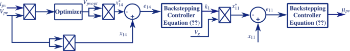
Control block diagram of the PV generation system.
Proposition 1
Consider the PV generation system modeled by the state-space equations (1a)-(1d) with the control input defined in (12), where \(c_{11}\), \(c_{12}\), and \(c_{13}\) are positiveidesign parameters. If the reference signal \(x_{11}^{*} = kV{g}\)iand its derivative exist,ithe system exhibits the followingiproperties:
-
1.
Theiclosed-loopidynamics of the variables (\(e_{11}\), \(e_{12}\), \(e_{13}\)) are governed by:
$$\begin{aligned} \begin{aligned} \dot{e}_{11}&= -c_{11}e_{11} + e_{12}, \\ \dot{e}_{12}&= -c_{12}e_{12} – e_{11}, \\ \dot{e}_{13}&= -c_{13}e_{13}. \end{aligned} \end{aligned}$$
(15)
This linear closed-loopisystem (15) is globallyiasymptoticallyistable under any initialiconditions. As a result, the PFC objective is asymptotically satisfied on average.
-
2.
Moreover, if \(k_1\)iconvergesito a finite value,ithe trackingierror of the PV voltage, \(\dot{e}_{14} = \dot{x}_{14} – \dot{x}_{14}^*\), follows the differential equation \(\dot{e}_{14} = -c_{14}e_{14}\), where \(c_{14}\) is aipositiveiconstant. Consequently, the closed-loop system achieves global exponential stability, ensuring that the error \(e_{14}\) decays exponentially regardless of the initial conditions. This guarantees that the PV voltage accurately tracksithe referenceivoltage providedibyioptimizer.
Wind power inverter controller design
The current \(x_{21}\) is required to track a reference \(x_{21}^{*}\) that is sinusoidal and proportional to the voltage \(V_g\), expressed as:
$$\begin{aligned} x_{21}^{*} = k_2V_g \end{aligned}$$
(16)
To achieve this objective, in the same way as before and by the same method. The backstepping controller is implemented in three steps.
Step 1: Define the tracking error as:
$$\begin{aligned} e_{21} = x_{21} – x_{21}^{*} \end{aligned}$$
(17)
From equation (17), the error dynamics can be expressed as:
$$\begin{aligned} \dot{e}_{21} = \frac{x_{22}}{L_g} – \frac{V_g}{L_g} – \dot{x}_{21}^* \end{aligned}$$
(18)
To stabilize the system, consider the quadratic Lyapunov function:
$$\begin{aligned} V_{21} = 0.5e_{21}^2 \end{aligned}$$
(19)
The time derivative \(\dot{V}_{21}\) becomes negative definite if the virtual input \(x_{22}\) is chosen as follows:
$$\begin{aligned} x_{22}^* = L_g(-c_{21}e_{21} + \frac{V_g}{L_g} + \dot{x}_{21}^{*}) \end{aligned}$$
(20)
where \(c_{22}\) is a positive design parameter. When \(x_{22}\) converges to \(x_{22}^*\), the error \(e_{21}\) evolves as \(\dot{e}_{21} = -c_{11}e_{21}\).
Step 2: Define the tracking error for \(x_{22}\):
$$\begin{aligned} e_{22} = x_{22} – x_{22}^{*} \end{aligned}$$
(21)
The corresponding dynamics is given by:
$$\begin{aligned} \dot{e}_{22} = -\frac{1}{C_{f2}}x_{23} – \frac{1}{C_{f2}}x_{21} – \dot{x}_{22}^* \end{aligned}$$
(22)
Using the Lyapunov function:
$$\begin{aligned} V_{22} = 0.5e_{22}^2 \end{aligned}$$
(23)
and selecting the virtual input \(x_{23}\) as:
$$\begin{aligned} x_{23}^* = C_{f2}(c_{22}e_{22} – \frac{1}{C_{f2}}x_{21} – \dot{x}_{22}^*) \end{aligned}$$
(24)
where \(c_{22}\) is a positive design parameter, \(\dot{V}_2\) becomes negative definite, ensuring system stability.
Step 3: Similarly, define the tracking error for \(x_{23}\) as:
$$\begin{aligned} e_{23} = x_{23} – x_{23}^* \end{aligned}$$
(25)
A Lyapunov function \(V_{23} = 0.5e_{23}^2\) is chosen, and the stabilizing control law is defined as:
$$\begin{aligned} \mu _{w} = \frac{L_{f2}}{V_{w}}(-c_{23}e_{23} + \frac{x_{22}}{L_{f2}} + \dot{x}_{23}^*) \end{aligned}$$
(26)
where \(c_{23}\) is a positive parameter, guaranteeing global stability of the system.
For the wind turbine voltage, the tracking error is defined as:
$$\begin{aligned} e_{24} = x_{24} – x_{24}^* \end{aligned}$$
(27)
Using a Lyapunov function \(V_{24} = 0.5e_{24}^2\), the stabilizing control law for the ratio \(k_2\) is given by:
$$\begin{aligned} k_2 = \frac{1}{V_g^2}\Big [\frac{C_{iw}}{2}(c_{24}e_{24} – \dot{x}_{24}^*) + \sqrt{x_{24}}i_{rec}\Big ] \end{aligned}$$
(28)
where \(c_{24}\) is a positive design parameter.
Figure 6 presents the control block diagram illustrating the strategy adopted for the wind energy generation system. This graphical representation complements the mathematical formulation by clarifying the role of the control variables and showing the coordination of the regulation loops, thereby facilitating the understanding of the operation of this subsystem within the overall microgrid.
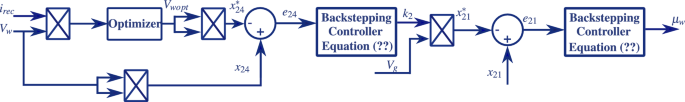
Control block diagram of the wind power generation system.
Proposition 2
Consider the wind power generation system modeled by the state-space equations (2a)-(2d) with the control input defined in (26), where \(c_{21}\), \(c_{22}\), and \(c_{23}\) are positive designiparameters.iIf theireference signal \(x_{21}^{*} = kV{g}\)iand itsiderivative exist,ithe system exhibits the followingiproperties:
-
1.
Theiclosed-loop dynamics of the variables (\(e_{21}\), \(e_{22}\), \(e_{23}\)) are governed by:
$$\begin{aligned} \begin{aligned} \dot{e}_{21}&= -c_{21}e_{21} + e_{22}, \\ \dot{e}_{22}&= -c_{22}e_{22} – e_{21}, \\ \dot{e}_{23}&= -c_{23}e_{23}. \end{aligned} \end{aligned}$$
(29)
This linear closed-loopisystem (29) is globallyiasymptoticallyistable under any initialiconditions. As a result, the PFC objective is asymptotically satisfied on average.
-
2.
Moreover, if \(k_2\) convergesito aifinite value, the trackingierror of the wind turbine voltage, \(\dot{e}_{24} = \dot{x}_{24} – \dot{x}_{24}^*\), follows the differential equation \(\dot{e}_{24} = -c_{24}e_{24}\), where \(c_{24}\) is a positive constant. Consequently, the closed-loop system achieves global exponential stability, ensuring that the error \(e_{24}\) decays exponentially regardlessiof the initialiconditions. This guarantees that the wind turbine voltage accurately tracks theireference voltageiprovided by ioptimizer.
Energy Storage inverter controller design
The current \(x_{31}\) is required to track a reference \(x_{31}^{*}\) that is sinusoidal and proportional to the voltage \(V_g\), expressed as:
$$\begin{aligned} x_{31}^{*} = k_3V_g \end{aligned}$$
(30)
To achieve this goal, define the tracking error as:
$$\begin{aligned} e_{31} = x_{31} – x_{31}^{*} \end{aligned}$$
(31)
From equation (31), the error dynamics can be expressed as:
$$\begin{aligned} \dot{e}_{31} =- \frac{V_{g}}{L_{f3}} – \mu _{b}\frac{\sqrt{x_{32}}}{L_{f3}} – \dot{x}_{31}^* \end{aligned}$$
(32)
A Lyapunov function \(V_1 = 0.5e_{31}^2\) is chosen, and the stabilizing control law is defined as:
$$\begin{aligned} \mu _{b} = \frac{L_{f3}}{\sqrt{x_{32}}}(-c_{31}e_{31} + \frac{V_{g}}{L_{f3}} + \dot{x}_{31}^*) \end{aligned}$$
(33)
where \(c_{31}\) is a positive parameter, guaranteeing global stability of the system.
The control design of the inverter will be conducted to ensure the charging and discharging of the battery. These two modes are known as CC mode and CV mode.
CC mode controller design
Recall that the control objective in CC mode is to enforce the battery current \(i_{b}\) to track its desired constant value \(i^*_{b}\). Using the backstepping design technique, it follows from the subsystem (3a–3c). Let first consider the following assumption:
Assumption 1
Knowing that the battery open circuit voltage \(U_{ocv}\) has a slow change rate compared with the battery current dynamics. So one can assume that \(\dot{U}_{ocv}\approx 0\). Let us introduce the battery current tracking error:
$$\begin{aligned} e_{32}=i_{b}-i_{b}^*=\frac{x_{32}-x_{33}-U_{ocv}}{R_{s}}-i_{b}^* \end{aligned}$$
(34)
In view of equation (34), the dynamic of the above error undergo the following differential equation:
\(\dot{e}_{32}=\frac{\dot{x}_{32}-\dot{x}_{33}}{R_{s}}=-\frac{\dot{x}_{33}}{R_{s}}+\frac{\dot{x}_{32}^2}{2{x}_{32}R_{s}}\)
wich gives:
$$\begin{aligned} \dot{e}_{32}=-\frac{\dot{x}_{33}}{R_{s}}+\frac{k_{3cc}V_g^2-i_{b}\sqrt{x_{32}}}{R_{s}C_{ib}\sqrt{x_{32}}} \end{aligned}$$
(35)
Using a Lyapunov function \(V_2 = 0.5e_{32}^2\), the stabilizing control law for the ratio \(k_{3cc}\) is given by:
$$\begin{aligned} k_{3cc} = \frac{1}{V_g^2}\Big [R_{s}C_{ib}\sqrt{x_{32}}[-c_{32}e_{32}+\frac{\dot{x}_{33}}{R_{s}}]+i_{b}\sqrt{x_{32}}\Big ] \end{aligned}$$
(36)
where \(c_{32}\) is a positive design parameter.
CV mode controller design
In this subsection, the control objective is to maintain the battery voltage \(V_{b}\) and equal to its constant reference \(V_{b}^*\) during the CV mode. Again, using the backstepping tecchnique, its follows from the subsystem (3a–3c), let us introduce the voltage tracking error as follows:
$$\begin{aligned} e_{33}=x_{32}-V_{b}^{2*} \end{aligned}$$
(37)
Considering that \(\dot{V}_{b}^{2*}=0\) and using equation (3b), the time derivation of equation (37) yields:
$$\begin{aligned} \dot{e}_{33}=\dot{x}_{32}=\frac{2}{C_{ib}}[k_{3cv}V_g^2-i_b\sqrt{x_{32}}] \end{aligned}$$
(38)
Using a Lyapunov function \(V_3 = 0.5e_{33}^2\), the stabilizing control law for the ratio \(k_{3cv}\) is given by:
$$\begin{aligned} k_{3cv} = \frac{1}{V_g^2}\Big [-\frac{C_{ib}}{2}c_{33}e_{33}+i_b\sqrt{x_{32}}\Big ] \end{aligned}$$
(39)
The control block diagram of the BESS, shown in Fig. 7, illustrates the adopted strategy, with particular emphasis on the selection between the CC and CV charging modes according to the battery SOC. This representation complements the mathematical formulation by explicitly defining the role of each control variable and clarifying the interaction between the regulation loops, thereby enhancing the understanding of the BESS charging and discharging processes as well as its contribution to the overall operation of the microgrid.
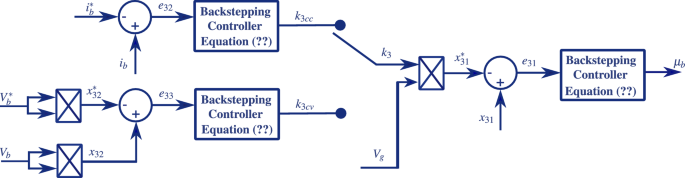
Control block diagram of the BESS.