
Our dataset of 64 whole-genome sequences captures a broad spectrum of B. burgdorferi s.s. genetic diversity within Canada. It includes 33 sequence types (STs), representing over one-third of the 90 known STs in the country, covering major genomic lineages circulating in different regions. Additionally, the dataset incorporates 22 ospC major groups and subgroups (out of 32 described in Canada), along with 10 intergenic spacer (IGS) types, 12 ribosomal spacer patterns (RSPs), and 3 restriction site types (RSTs). All samples were collected in 2016, minimizing potential temporal bias. While our aim was to capture the overall genetic diversity present in Canada, the dataset was not designed to exhaustively represent the full diversity within each individual region.
Comparative phylogenetic analysis of partitioned and concatenated evolutionary models
To evaluate the impact of different evolutionary models on phylogenetic inference, we compared partitioned and concatenated models of all chromosomal markers (BmpA, FlaB, oms66, P83-100, clpA, clpX, nifS, pepX, pyrG, recG, rplB, uvrA and rrs-rrlA) using IQ-TREE (Fig. S1 and S2). The phylogenetic inference using partitioned and concatenated evolutionary models revealed identical tree topologies, with only minor differences in node support values (Fig. S1, S2). Notably, the only topological difference was observed when comparing the concatenated GTR model (Fig. S2) to the Jukes-Cantor (JC) model (Fig. 1): in the JC tree, Groups 1 and 2 formed a single monophyletic cluster, whereas in the GTR tree, they appeared as two distinct, well-supported clades. This difference arises because the JC model assumes equal substitution rates among all nucleotide changes, making it less sensitive to subtle differences between lineages. As a result, the JC model groups closely related but distinct clades (Groups 1 and 2) into a single cluster with internal substructure. In contrast, the GTR model accounts for variable substitution rates across sites (i.e., it still allows different substitution rates between nucleotides), allowing finer resolution and clearer separation of these groups into distinct clades with stronger statistical support.
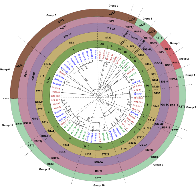
Global maximum likelihood phylogenetic tree of concatenated nucleotide sequences from 13 chromosomal markers of B. burgdorferi sensu stricto (BmpA, FlaB, oms66, P83-100, clpA, clpX, nifS, pepX, pyrG, recG, rplB, uvrA, and the 16–23 S intergenic spacer). Isolates are color‑coded by geographic region: Manitoba (MB, blue), Ontario (ON, green), and Nova Scotia (NS, brown). Colored circle bands indicate genetic markers: ospC major groups (bold green), ribosomal sequence types (RST1, red; RST2, brown; RST3, light green), multilocus sequence types (STs, yellow), intergenic spacer (IGS) subtypes (purple), and ribosomal spacer patterns (RSPs, pink). Twelve numbered clades represent well‑supported phylogenetic groups and isolates not clustering within these monophyletic groups were annotated as singletons.
Our results (Table S3) indicate that the Robinson-Foulds (RF) distance between the partitioned and concatenated models was minimal (RF distance = 10, normalized RF distance = 0.0769), suggesting strong topological consistency between both approaches. When benchmarked against the core genome phylogeny, the concatenated model achieved a lower normalized RF distance (0.2769) than the partitioned model (0.3385), indicating higher congruence with the core genome. Log-likelihood values were nearly identical between models (− 22557.732 versus − 22557.785), with ΔlogL = 0.052. However, likelihood-based tests – Shimodaira-Hasegawa (p-SH = 1.0 versus 0.0231), Kishino-Hasegawa (p-KH = 0.974 versus 0.0259), and approximate unbiased (p-AU = 0.976 versus 0.0235), strongly favored the concatenated model and statistically rejected the partitioned approach.
Taken together, these results support the validity of concatenation for phylogenetic reconstruction in B. burgdorferi s.s., demonstrating that a single evolutionary model across all genes (i.e., chromosomal genes) provides robust and reliable topologies comparable to partitioned approaches, while improving computational efficiency.
Phylogenetic tree comparison and congruence analysis
The core genome phylogenetic tree constructed in MEGA 5.2.237 with the Jukes-Cantor (JC) model revealed that concatenating sequences of bmpA, flaB, oms66, P83-100, eight housekeeping genes (clpA, clpX, nifS, pepX, pyrG, recG, rplB, uvrA), and the 16–23 S chromosomal marker, divided 59 of the 64 B. burgdorferi s.s. strains into 12 well-supported monophyletic groups that were also classified based on MLST, IGS, RSP, and RST markers. Group delineation was based either on the most recent common ancestor (MRCA) with high bootstrap support (≥ 0.95) or, in cases where a larger clade contained well-resolved subclades, on the consistency of those subclades with one or more independent typing methods (MLST, ospC MG, IGS, RSP, RST). The other five strains were singletons (Fig. 1). While higher-order branching patterns sometimes differed between core genome and plasmid-gene trees, the internal monophyly of each group was preserved across datasets. Branch lengths in the phylogenetic tree are proportional to nucleotide divergence, allowing inference of relative evolutionary distances among and within clades. These phylogenetic groups and their respective geographic distributions, based on the sequence types (STs) reported in the pubmlst.org database (Table S4), are as follows:
-
• Group 1 (ST55, IGS-1 A, RSP2, RST1): ST55 is found in the Midwestern USA (Minnesota, Wisconsin) and south central Canada (Manitoba, Ontario).
-
• Group 2 (ST1, IGS-1 A, RSP1, RST1): ST1 is predominantly distributed in the Northeastern USA (Connecticut, Massachusetts, Maine, New Hampshire, New York, Pennsylvania, Rhode Island, Virginia, Vermont) and central and southeastern Canada (Ontario, Quebec, and the Maritimes).
-
• Group 3 (ST46, IGS-8 C, RSP13, RST3): ST46 is found in the Midwestern USA (Wisconsin, Minnesota) and south central Canada (Ontario, Manitoba).
-
• Group 4 (ST51, ST268, IGS-5, RSP14): STs 51 and 268 are found in the Northeastern and upper Midwestern USA (Minnesota, Wisconsin, New York) and central and western Canada (Manitoba, British Columbia).
-
• Group 5 (ST3, IGS-2 A, RSP3, RST2): ST3 is primarily found in the Northeastern USA (Massachusetts, New York, Connecticut, Vermont, Virginia, Rhode Island, New Jersey) and southeastern Canada (Maritimes, Ontario, Quebec).
-
• Group 6 (ST4, ST32, ST740, IGS-2D, RSP4, RST2): STs 4, 32 and 740 are distributed across the Northeastern and Midwestern USA (Connecticut, Illinois, Massachusetts, Maine, Michigan, Minnesota, New Jersey, New York, Pennsylvania, Rhode Island, Wisconsin) and southern Canada (Manitoba, Ontario, Quebec, and the Maritimes).
-
• Group 7 (ST29, IGS-2D, RSP5, RST2): ST29 is found in the Northeastern and Midwestern USA (Connecticut, Illinois, Minnesota, Wisconsin) and across southern Canada (British Columbia, Manitoba, Ontario, Quebec).
-
• Group 8 (ST530, IGS-2D, RSP5, RST2): ST530 was identified in the upper Midwestern USA (Wisconsin, Minnesota) and south central Canada (Manitoba, Northwestern Ontario).
-
• Group 9 (ST16, ST227, ST237, ST741, IGS-7 A, RSP10, RST3): STs 16, 227, 237 and 741 are distributed across the Northeastern and upper Midwestern USA (Connecticut, Massachusetts, New York, Rhode Island, Wisconsin) and across southern Canada (British Columbia, Manitoba, Ontario, Quebec, and the Maritimes).
-
• Group 10 (ST12, ST221, IGS-6 A, RSP9, RST3): STs 12 and 221 are found in northeastern and upper Midwestern USA (Connecticut, Massachusetts, New York, Rhode Island, Wisconsin, Michigan, Illinois) and across southern Canada (British Columbia, Manitoba, Ontario, Quebec, and the Maritimes).
-
• Group 11 (ST43, IGS-5, RSP14, RST3): ST43 is found in the upper Midwestern USA (Wisconsin, Minnesota) and western and south central Canada (British Columbia, Manitoba, Northwestern Ontario).
-
• Group 12 (ST19, ST31, ST229, IGS9, RSP19, RST3): STs 19, 31 and 229 are distributed across the Northeastern and upper Midwestern USA (Connecticut, New York, US Midwest) and south central and southeastern Canada (Manitoba, Ontario, Quebec, and the Maritimes).
Notably, several core phylogenetic groups correspond to unique combinations of ST, IGS, and RSP types, such as Group 1 (ST55, IGS-1 A, RSP2, RST1), Group 2 (ST1, IGS-1 A, RSP1, RST1), and Group 5 (ST3, IGS-2 A, RSP3, RST3) (Table S3). This classification provides a framework for understanding the evolutionary relationships of B. burgdorferi s.s. strains. Seven strains had unique combinations of MLST, IGS, RSP, and RST types (Fig. 1).
Congruence across classification methods
To assess the consistency between core and plasmid-encoded genes, congruence was calculated between these core genome groups and the plasmid gene trees (Figures S3–S13) for ospC, dbpA, dbpB, oms28, ospA, ospB, ospD, Fibronectin P35, P37, P45-13 and C6 peptide of vlsE1 using different classification methods (Tables S5-S9). The tables provide a quantitative summary of the visual comparisons shown in Figures S3–S13, converting tree‑based congruence into a binary scoring system to facilitate direct comparison.
MLST classification
The MLST classification method consistently exhibited high congruence with the core genome tree across most phylogenetic groups. Notably, Group 1 (ST55), Group 2 (ST1), Group 3 (ST46), and Group 8 (ST530) achieved a high congruence (91%-100%) across all genes, indicating strong evolutionary coherence (Table S5). Fibronectin P35 showed high congruence (91%), indicating its stable alignment with the core genome. Similarly, dpbA, dpbB, and ospC also demonstrated high congruence (75%), reflecting their phylogenetic alignment with core genome markers. Conversely, ospA exhibited the lowest congruence (27%).
OspC major group classification
The major ospC grouping was variably congruent with the core genome and other plasmid markers. The C6 peptide of VlsE1 achieved the highest congruence (100%), followed by ospC (75%) and P45-13 (73%), indicating strong alignment between these genes and the core genome. However, Group 1 (ST55, ospC A) showed a lower congruence score (55%) compared to Group 2 (ST1, ospC A) at 73%, indicating differences in phylogenetic consistency between these groups. Genes like ospA (27%) and oms28 (42%) had lower congruence with ospC (Table S6).
IGS classification
The IGS classification method was poorly congruent with other markers. The C6 peptide showed the highest congruence with IGS (67%) across groups, particularly in Groups 3, 5, 8, 10 and 12. Other genes, such as Fibronectin P35 (18%) and ospA (18%), exhibited low congruence with core genome (Table S7).
RSP classification
The RSP classification method demonstrated moderate to high congruence with other markers. Groups 1, 3, and 8 RSP were > 78% congruent with ospD, C6, and P37, but RSP classification was poorly congruent with the ospA (36%) (Table S8).
RST classification
The RST classification method displayed the lowest overall congruence scores. dpbA, dpbB, oms28, ospC, and ospD showed minimal congruence with RST classification (respectively 17%, 33%, 8%, 17%, 25%), while others like ospA, ospB, Fibronectin P35, P45-13 and P37 exhibited no congruence (0%) (Table S9).
Group-level insights and general observations
Groups 1, 2, 3, and 8 showed the highest congruence scores across multiple classification methods, suggesting they form stable, monophyletic clades. Notably, Group 8 (ospC allele C3) exhibited high evolutionary stability across genes – but this is a very small group (only 2 strains). Conversely, Group 2 (ST1, ospC A) showed lower congruence compared to Group 1 (ST55, ospC allele A) (Fig. S3–S13).
Across all classification methods, MLST and ospC major groups displayed the highest overall congruence. In contrast, RST classification consistently showed the lowest congruence.
General insights across classification methods
The MLST and ospC major group classification methods demonstrated the highest overall congruence with the core genome. Genes such as, C6 peptide of vlsE1, and dbpA consistently showed high congruence across multiple methods (Fig. S3–S13). Conversely, ospA and P45-13 consistently exhibited lower congruence across all classification methods. The RST classification method demonstrated the lowest congruence across all genes.
Recombination versus mutation analysis
To understand the evolutionary forces shaping B. burgdorferi s.s. populations, we compared the impact of recombination versus mutation across the core genome and several plasmid-encoded genes using ClonalFrameML. The R/θ ratio, representing the relative contribution of recombination to mutation, revealed distinct patterns across different genomic regions. The core genome exhibited a moderately high R/θ ratio of 1.50 (Table 1), indicating that recombination plays a significant role in its evolution. However, while mutation contributes to genetic variation, its effects are generally more constrained compared to recombination, which can introduce larger-scale genomic changes. This relative constraint may help preserve the integrity of essential chromosomal regions.
Among the plasmid‑encoded antigens, recombination rates varied substantially: ospC showed the highest recombination relative to mutation (R/θ = 4.25), whereas ospA and P45‑13 exhibited markedly lower ratios, and ospB showed intermediate values (Table 1). These findings highlight the differential evolutionary pressures acting on major surface antigens.
Statistical analysis
Core genome and accessory gene relationships: To further investigate the degree of evolutionary consistency between core genome and accessory genes in B. burgdorferi s.s., we calculated the distance (as measure by % nucleotide divergence) of each gene, in every strain, to the homologue on the reference genome B31. We then checked for the strength of correlations in these distances between different pairs of genes (Table 2). Significant positive correlations were found between the C6 peptide and chromosomal genes: bmpA (r = 0.76, R² = 0.58, p < 0.001), flaB (r = 0.63, R² = 0.4, p < 0.001), and sequence types (ST) (r = 0.81, R² = 0.65, p < 0.001), IGS (r = 0.81, R² = 0.65, p < 0.001), RSP (r = 0.54, R² = 0.3, p = 0.003), and RST (r = 0.57, R² = 0.32, p = 0.002) (Table 2). Similarly, dbpA showed moderate positive correlations with bmpA (r = 0.6, R² = 0.35, p < 0.001), flaB (r = 0.55, R² = 0.31, p < 0.001), and ST (r = 0.59, R² = 0.34, p < 0.001). Negative correlations revealed potential evolutionary divergence. ospC showed negative correlations with oms66 (r = -0.39, R² = 0.15, p = 0.002) and P83-100 (r = -0.35, R² = 0.12, p = 0.005) (Table 2). Similarly, oms28 was negatively correlated with flaB (r = -0.3, R² = 0.09, p = 0.018).
Hierarchical clustering analysis
To further examine how different genes reveal consistent patterns of sequence similarity to the B31 reference genome, hierarchical clustering analysis was performed using Euclidean distance and single-linkage methods. This analysis allowed us to visualize how the degree of similarity to the B31 reference genome translated into phylogenetic relationships among the core and accessory genomes. Strains carrying ospC alleles I (i.e., including Ia subtype) and K consistently formed monophyletic clades in both core and accessory genome trees, as confirmed by maximum likelihood (ML) phylogenetic trees with high bootstrap support values (1 for ospC I-Ia and 0.99 for ospC K) (Fig. S3). These clusters aligned with the positive correlations observed between ospC and markers like RSP (r = 0.47, R2 = 0.22, p < 0.001) and RST (r = 0.44, R2 = 0.19, p = 0.001) (Table 2).
However, negative correlations between ospC and core proteins such as oms66 were reflected in phylogenetic splits. The hierarchical clustering analysis revealed that strains carrying ospC I-Ia (Fig. 2A and B) were divided into two distinct clusters. A similar pattern was observed with ospC K (Fig. 2A and C), where the negative correlation with P83-100 resulted in a phylogenetic split.

Hierarchical dendrograms illustrating relationships between the plasmid gene ospC and selected chromosomal genomic markers in Borrelia burgdorferi sensu stricto. Panels show: (A) ospC vs. FlaB (positive correlation), (B) ospC vs. oms66 (negative correlation), and (C) ospC vs. P83-100 (negative correlation). The dendrograms include all 64 Canadian strains, with ospC molecular genotypes (MGs) labeled. Genotypes influenced by negative correlations are highlighted with red circles. The colors in the dendrogram denote distinct clusters.
Degree of clonality and modularity of B. burgdorferi
To assess the degree of clonality in B. burgdorferi s.s. populations from different geographic regions (NS, ONMB), we compared the ratio of haplotypes to singletons. Ontario and Manitoba were combined due to the lack of significant statistic differences in their B. burgdorferi s.s. population clonality (data not shown). A Mann-Whitney U test revealed a statistically significant difference in clonality, measured as haplotype-to-singleton ratios, between the B. burgdorferi s.s. populations in Nova Scotia (NS) and the combined Ontario/Manitoba (ONMB) regions (U = 975, p < 0.001) showing that the degree of clonality is higher in NS compared to ONMB (Table 3).
Cliff’s Delta had a value of + 1, indicating all clonality ratios in NS were greater than those observed in ONMB, supporting the interpretation that the NS population demonstrates a consistently higher level of clonality relative to ONMB (Table 3).
Network analysis: To uncover regional patterns in population structure, we conducted network-based modularity and association analyses across the three regions: Nova Scotia (NS), Ontario (ON), and Manitoba (MB). In this analysis, we treated Ontario and Manitoba separately, unlike in the clonality analysis where they were grouped together. This distinction was made because clonality measures genetic redundancy within a population, whereas modularity assesses the presence of distinct genetic clusters (subpopulations) within a region. Since ON and MB share many strain types, it made sense to group them for clonality analysis. However, for modularity analysis, we observed regional genetic differentiation, with some groups being exclusive to Manitoba (Groups 3, 4, 7) and others to Ontario (Group 11), which warranted separate analyses.
The modularity index (Q) confirmed moderate to strong community structures across all regions. The Nova Scotia (NS) population had the highest modularity (Q = 0.68), indicating well-defined genetic clusters. In contrast, Ontario exhibited the lowest modularity (Q = 0.508), suggesting a more fragmented and mixed population structure, while Manitoba had an intermediate modularity value (Q = 0.634), reflecting moderate population structuring.
Beyond clustering, our network analysis highlighted clear genetic associations between B. burgdorferi s.s. strains in Nova Scotia, Ontario, and Manitoba and their respective reference strains, alongside shared genomic markers. Seven of the 12 monophyletic groups identified in Nova Scotia were closely related to reference strains, suggesting that these strains share a common evolutionary history while also displaying regional genetic divergence (Fig. 3). For example, Group 2 was genetically identical to the B31 reference strain, suggesting a direct lineage connection, while Group 5 showed similarities with B379 and 297, and Group 6 was closely related to the 156a strain. Group 12 exhibited genetic proximity to N40, reflecting a shared evolutionary background. The network analysis revealed distinct genetic associations between B. burgdorferi s.s. strains and reference strains across different regions, providing insights beyond core genome-based phylogenies. In Ontario, Groups 1, 8, 9, 10, and 11 aligned closely with reference strains 156a, ZS7, B331, 29,805, WI91-23, and N40 (Fig. 4), supported by genetic markers such as IGS-1 A (Group 1) and IGS-2D/RSP5 (Group 8). In Manitoba, nine of the twelve groups displayed distinct relationships, with Groups 6 and 7 associating with 94a, JD1, and 118a, while Groups 4 and 12 aligned with CA11-2 A and WI91-23 (Fig. 5). In Nova Scotia, Groups 2 and 5 were exclusive to this region, with Bb163 from Group 2 being genetically identical to the B31 reference strain. Notably, the same phylogenetic group sometimes aligned with different reference strains depending on the region; for instance, Group 1 aligned with 156a in Ontario but ZS7, 118a, and B331 in Manitoba. This network-based approach complements phylogenetic trees by incorporating gene-specific alignments, particularly for plasmid genes, which are not fully captured in core genome-based phylogenies.

Network graph illustrating genetic relationships among 26 Borrelia burgdorferi sensu stricto strains collected in Nova Scotia, Canada. Relationships are based on a comprehensive set of chromosomal and plasmid-encoded genomic markers. Chromosomal markers include BmpA (P39), FlaB (P41), oms66 (P66), and P83-100 (P83), together with eight housekeeping genes (clpA, clpX, nifS, pepX, pyrG, recG, rplB, uvrA) and the C6 peptide of VlsE1. Plasmid-encoded markers include dbpA (P17), dbpB (P18), fibronectin-binding protein (P35), oms28 (P28), ospA (P31), ospB (P34), ospC (MG), ospD (P30), P37, and P45-13 (P45). Strain nodes are color-coded by sampling location: yellow for Bedford, black for Lunenburg, red for Pictou, and green for Shelburne. Genomic marker nodes are shown in cyan. Black edges represent the highest sequence similarity scores, as determined by BLAST analysis, indicating genetic connections among strains based on shared markers.

Network graph illustrating genetic relationships among 26 Borrelia burgdorferi sensu stricto strains collected in Ontario, Canada. Relationships are based on a comprehensive set of chromosomal and plasmid-encoded genomic markers. Chromosomal markers include BmpA (P39), FlaB (P41), oms66 (P66), and P83-100 (P83), together with eight housekeeping genes (clpA, clpX, nifS, pepX, pyrG, recG, rplB, uvrA) and the C6 peptide of VlsE1. Plasmid-encoded markers include dbpA (P17), dbpB (P18), fibronectin-binding protein (P35), oms28 (P28), ospA (P31), ospB (P34), ospC (MG), ospD (P30), P37, and P45-13 (P45). Strain nodes are color-coded by sampling location: green for Big Grassy, black for Big Island, brown for Birch Island, and blue for Manitou Rapids. Genomic marker nodes are shown in yellow. Orange edges represent the highest sequence similarity scores, as determined by BLAST analysis, indicating genetic connections among strains based on shared markers.

Network graph illustrating genetic relationships among 26 Borrelia burgdorferi sensu stricto strains collected in Manitoba, Canada. Relationships are based on a comprehensive set of chromosomal and plasmid-encoded genomic markers. Chromosomal markers include BmpA (P39), FlaB (P41), oms66 (P66), and P83-100 (P83), together with eight housekeeping genes (clpA, clpX, nifS, pepX, pyrG, recG, rplB, uvrA) and the C6 peptide of VlsE1. Plasmid-encoded markers include dbpA (P17), dbpB (P18), fibronectin-binding protein (P35), oms28 (P28), ospA (P31), ospB (P34), ospC (MG), ospD (P30), P37, and P45-13 (P45). Strain nodes are color-coded by sampling location: green for Buffalo Point and blue for Roseau River. Genomic marker nodes are shown in peach. Brown edges represent the highest sequence similarity scores, as determined by BLAST analysis, indicating genetic connections among strains based on shared markers.