
To illustrate what an extreme ET event is, we first consider the seven days of every year when a region in Central Western Europe experienced the highest cumulative ET (ETx7d) in ERA5 Land (Fig. 1). We highlight the years with the strongest (2019) and second strongest (2022) ETx7d events. These seven days are commonly associated with little to no precipitation, as well as high incoming short-wave radiation. In addition, temperatures tend to be high and the relative humidity low, leading to a high vapor pressure deficit. In the mid latitudes, these conditions are often associated with high surface pressure, but this is not necessarily found in tropical regions such as eastern Brazil (Fig. S6). These events result in strong decreases in soil moisture.
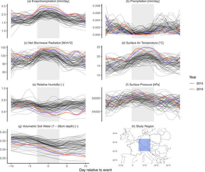
The x-axis indicates days relative to the event, with 0 being the center of the 7-day event. The gray box indicates the 7-day duration based on which the events were selected. The variables shown are a evapotranspiration, b precipitation, c net short wave radiation, d surface air temperature, e relative humidity, f surface pressure, and g volumetric soil water. Two lines are colored and indicate the strongest (2019) and second strongest (2015) events in the study region (h). The other lines indicate the evolution of all other events between 1950 and 2023. A loess smoother was applied to improve visual clarity.
The evolution of these variables points to a heat wave as the common driver, which matches our physical expectation of such an event31. The two strongest events over Europe are characterized by very high short-wave radiation, low relative humidity, and high temperatures. We also find these features in other regions, like eastern Brazil (Fig. S6) and the central US (Fig. S5). In dryer regions like the central US, we also see a preconditioning on water availability. The two strongest events occurred at relatively high soil moisture leading into the event. In contrast, the year 2012, which was associated with a strong drought, had one of the smallest ETx7d values. In the European study region, the two strongest events occurred very recently, suggesting an increase in ETx7d. We therefore want to investigate whether we find this tendency towards increasing ETx7d with CMIP6 models.
Event intensity in CMIP6
For this, we first consider the evolution of the intensity of an ETx7d event in climate models forced with the historical and then the SSP5-8.5 emission scenario in the European SREX regions (Fig. 2). In the Mediterranean, most climate models show a decrease of ETx7d intensity up to 1980, with the exception of CESM2, where the intensity increases up to around 2030. The period between 1950 to 1980 is associated with high aerosol emissions, which dims short-wave radiation and thus limits ET. The subsequent reduction in aerosol emissions and therefore increased short-wave radiation, most models show an increase in ETx7d. Event intensity in UKESM1-0-LL remains low and never recovers to levels of 1850. Although the models span a wide range of responses, the observations agree on an increase, after a local minimum around the year 2000. However, hydrological variability is particularly large in this region32 and trends should be interpreted with caution. In Western Central Europe (WCE), the models behave similarly to those in the Mediterranean. The increase in ETx7d intensity after 1980 is more pronounced, but so is a decline starting in 2020. CESM2 again shows no local minimum, and ETx7d increases continuously until 2050. However, all models agree on an increase in ETx7d between 1980 and 2020. The decrease, which all models show, is likely tied to water limitations emerging towards the end of the century in a high-emission scenario33. The observations all agree on very strong increases starting in 1980, which again points to the importance of aerosol-induced changes. ETx7d in northern Europe decreases slightly during the period of high aerosol emissions in Europe, reaches a minimum in most models around 1980 and then increases above the levels early in the simulations. MPI-ESM1-2-HR and CESM2 show slight decreases after 2050 in ETx7d, while the other three models show steady increases. However, the evolution over time is very comparable between climate models. The trends in the observational products are not as strong as for WCE but seem to intensify towards the most recent years.
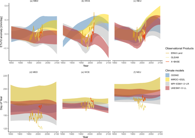
Anomalies are shown for the three European SREX regions Mediterranean Med (a), Western Central Europe WCE (b), and Northern Europe NEU (c). The shading shows a smoothed range of ± one standard deviation around the ensemble mean in a selection of climate models forced with the historical and subsequent SSP5-8.5 scenario. The lines represent the Ex7d in three observational products over these SREX regions with a three-year running mean applied for visual clarity. d, e, f show the timing as the day of the year when the maximum occurred in the same climate models and observations. Day 125 corresponds to 5 May and day 225 to 3 August.
Event timing in CMIP6
We would expect increasing water limitation to result in ETx7d events shifting towards earlier in the season, when there is more water available. However, this cannot be concluded from the data, as the timing of ETx7d events is subject to less clear and intense changes in general. In the Mediterranean, the climate models show a tendency towards events earlier in the season towards the end of the 21st century. The observations, but also the climate models, show substantial disagreement in the overall timing. Events in GLEAM and ERA5 Land tend to occur comparatively early in the season. The only climate model that shows similarly early extremes is MPI-ESM1-2-LR. Events in X-BASE occur later in the season, but still not as late as two of the climate models shown here. The reason for this large range in timings is likely caused by discrepancies in the strong seasonal cycle of ET. Since we are extracting the highest absolute values, they can realistically occur only during the peak of the seasonal cycle. Climate models have been shown to have discrepancies in the seasonal cycle of precipitation34, which will have the biggest impact in a more water-limited Mediterranean. In WCE, there is broader agreement on the timing of ETx7d events. Most climate models show a tendency towards earlier events towards the end of the 21st century, which again points towards water becoming an important limitation. GLEAM and ERA5 Land do not show great changes in the timing, in contrast to X-BASE, which sees a shift towards events earlier in the season. In Northern Europe, the climate models again show little change in the event timings. The observations lie at the lower end or even outside the range spanned by the climate models.
Overall, we see relatively broad agreement among climate models and observations on an increase in ETx7d intensity over the recent historical period, which we want to investigate on a larger spatial scale. We want to see whether a detectable shift in the distribution of ETx7d has been observed and whether such a shift is consistent with climate models.
Detecting changes in extreme ET
To detect a change in the observational data sets, we employ a detection and attribution technique based on a regularized regression model. The regression model predicts the ensemble mean ETx7d of a climate model from the ETx7d maps of only a single ensemble member. Such a regression setup results in a statistical model that is able to reduce the influence of internal variability but also accounts for some climate model disagreement, allowing for a more robust trend detection. In order to examine whether changes in the extremes are stronger than in the mean, we repeat the analysis for the mean ET of the Northern hemisphere of June, July and August (JJA) and the mean ET of the Southern hemisphere of December, January, and February (DJF). The coefficients of the regression models, shown in Fig. 3a, b, c, are mostly positive. They can be mapped out to their corresponding location, showing where the model is drawing information from. Grid cells that are assigned a large coefficient contribute more to the prediction of the forced response (FR). These grid cells are in regions where internal variability is comparatively low and where climate models agree most about their relationship with the ensemble mean. We do expect mostly positive coefficients, since the ensemble mean is positively correlated with the grid cells that underlie it. Using this regression model, we then predict the forced response for all the members of the climate models used and calculate the 1980–2023 trends forced with historical emissions. Additionally, we also predict the forced response in climate model simulations, which exclude anthropogenic activity (PiControl), to estimate the ranges of likely unforced trends (Fig. 3d, e, f). The unforced trends serve as a null distribution of trends that can emerge solely due to natural variability. The historical trends serve as the alternative hypothesis, representing the ranges of trends we can expect under anthropogenic activity. We then applied the regression model to the two observational data sets, GLEAM and ERA5 Land, to obtain an estimate of the observed FR, indicated by the vertical lines. The shading around the lines shows the range of one standard deviation from the mean trend, obtained by bootstrapping the years that are included in the trend estimation.
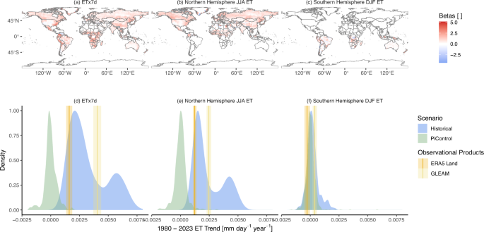
Mapped coefficients for predicting the forced response of global mean ETx7d (a), Northern (b), and Southern (c) hemisphere summer mean ET. The coefficients have been scaled to the same variance but not centered, so positive values indicate positive correlation with the forced response. ETx7d (d), Northern hemisphere JJA ET (e), and Southern hemisphere DJF ET (f) forced trend density of historical (blue) and PiControl (green) climate model simulations between 1980 and 2023. Observational trend of GLEAM and ERA5 Land is indicated by the vertical lines, as well as the bootstrapped standard deviation by the shading around the lines. Maps made with Natural Earth.
The ETx7d forced trend from ERA5 Land lies at the very upper end of the unforced trends and within the lower portion of the forced trends. The forced trend for GLEAM is larger and lies clearly outside the null distribution and well within the historical forced trends. For the Northern hemisphere JJA ET, the distributions look very similar. The trends of both observational products would be very unlikely in a preindustrial climate but well within the expected trends under historical greenhouse gas and aerosol emissions. It is also worth noting that we find a similarly robust signal of change in JJA ET and ETx7d. The observational products fall into similar quantiles of the historical and PiControl trend distribution for both JJA ET and ETx7d. The ETx7d trends are larger, but so is the range in the PiControl distribution, which reduces the signal-to-noise ratio. The observational trends of JJA ET are generally smaller, but so are the likely ranges of the PiControl trends.
The observational summer trends (DJF) in the Southern Hemisphere lie within the piControl distribution. However, the historical CMIP6 simulations also show no clear trend in either direction. Thus, we neither find nor expect a robust change in the Southern Hemisphere average.
Additionally, we repeated the analysis for global and seasonal mean ETx7d for the 2001 to 2021 time span, allowing the inclusion of X-BASE (Fig. S7). We also find a strongly detectable signal in all observational products for global and northern hemisphere JJA ETx7d, with X-BASE showing the largest change over the time period. For Southern hemisphere DJF ETx7d, we find no detectable changes.
Regional changes
To investigate more regional changes, we focus on the SREX regions defined in IPCC’s AR6. We calculate the weighted spatial mean ETx7d and JJA ET of all grid cells within a given SREX region and omit the regularized regression step, as the regularization offers little benefit over the spatial mean when estimating very regional FR. Thus, we calculate the 1980-2023 Theil-Senn trends for both ERA5 Land and GLEAM for ETx7d and JJA ET for all SREX regions over land (Fig. 4). Since changes are less robust during Southern hemisphere summer, we omit DJF ET from this analysis and only show it in the Supplementary (Fig. S2). We repeat the procedure for forced and unforced climate model simulations analogously to Fig. 3. To evaluate the consistency of trends across datasets and assess significance, we perform a series of tests for each region.
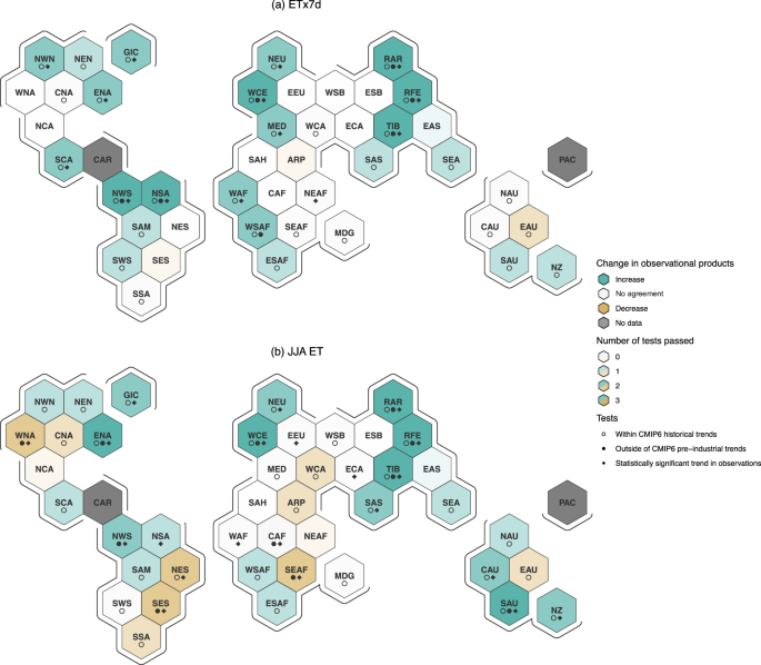
ETx7d trends are shown in (a) and JJA ET trends in (b) across all SREX regions over land. The color indicates regions where ERA5 Land and GLEAM agree on the sign of the 1980–2023 trend. The strength of the color indicates the number of the three tests a region passes. When these two trends lie within the distribution of CMIP6 historical trends, a circle is added to the region. When both observational trends lie outside the CMIP6 pre-industrial distribution, the black dot is added. Finally, when the observed trends both pass a Mann-Kendall significance test, the diamond is added.
Each hexagon is colored if the two observational datasets agree on the direction of change. This agreement occurs in slightly fewer than half of the regions for ETx7d. In contrast, for JJA ET, the observational data sets agree in most regions, with approximately two-thirds indicating an increase. Next, we test whether the two observational trends lie within the distribution of the historical simulations of CMIP6. Regions that pass this test are indicated with a circle, which is the case for almost every shaded region. Thus, observational products and climate models with historical emissions show trends that agree in many cases. We find significant trends (either outside the PiControl distribution or passing a Mann-Kendall test) for a number of regions. When a region passes both tests, it increases our confidence in the robustness of change in those regions. Note that an empty cell only indicates a lack of agreement on the observed trend sign, not agreement on the absence of a change. The strength of the coloring is determined by the number of tests passed, with stronger colors indicating increased confidence in significant changes.
A notable region is WCE, which passes all the tests for both ETx7d and JJA mean ET. Although the strong temperature trends over Europe have almost certainly helped to drive this trend, it is very likely to be superimposed on a trend of increased surface radiation over Europe in the last 40 years. This increase in surface radiation is known as global brightening driven by reduced aerosol emissions and concentrations as a result of air pollution measures35). Of course, there are also other processes that drive an increase in ET, such as greening. However, the regional strength of these changes does point towards a more regional driver, such as aerosol concentrations or dynamical trends, rather than a more global driver like temperature increase and greening. Regions in higher latitudes, such as NWN, NEU, RAR, and RFE, tend to show a clear tendency toward increases in both ETx7d and JJA ET. ET is expected to increase with increasing potential ET in regions with abundant water. The two regions that make up Northern South America also show increases in both ETx7d and JJA ET. Also worth noting are the JJA ET trends in Western North America, South-Eastern South America and South-Eastern Africa. The observed trends agree on a decrease, which is significant and outside the PiControl range but not within the historical CMIP6 distribution. Assuming that the observed trends are reliable, climate models do not capture the strong observed decreases in these regions. When comparing the two maps, it is worth noting that all regions that show an increase in ETx7d also show an increase in JJA ET, with the exception of the Mediterranean. This agreement could indicate that the trends in the extremes are mostly driven by the trend in the mean, where changes in the whole distribution led to higher values at the tail end. However, ETx7d trends are larger in most regions than the ones for JJA ET in the observations (Fig. S3) and climate models (Fig. S4), indicating an additional increase in variability in the distribution of ET. For the regions where JJA ET decreased, we universally find no robust change in ETx7d. This is likely caused by long-term decreases in water availability, which are less visible when focusing on high ET extremes. However, a decrease in the mean and no change in the extreme suggest an increase in the span of the distribution, as ETx7d moves further from the seasonal mean. A greater variance in precipitation and ET is the core process driving drought risk8. The divergence of mean and extreme ET can again be seen in Figs. S3 and S4, where regions with decreasing JJA ET show less change in ETx7d. In general, we can see the impact of anthropogenic climate change on the hydrological cycle even in ET products, and changes can be detected on a hemispheric and, in some cases, even regional scale. Repeating the analysis for the 2001 to 2021 period with the inclusion of X-BASE does not lead to new insights. The short trend estimation period in combination with the large internal variability on regional scale does not allow for the detection of robust trends (Fig. S8).
Record setting
We further highlight the strong changes in ETx7d in Europe by illustrating the year in which the record of a grid cell was set (Fig. 5).
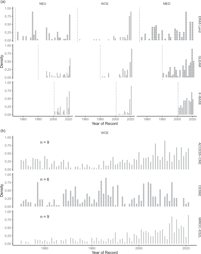
Panel a shows three observational products (ERA5 Land, GLEAM, X-BASE), and b three climate models (ACCESS-CM2, CESM2, MIROC-ES2L). A point represents a grid cells’s record being set in a given year. Europe is split up into the three regions Northern Europe (NEU), Western Central Europe (WCE), and Northern Europe (NEU). For each climate model, the number (n) ensemble members used in the analysis is noted in the panel.
All investigated observational products agree that a large number of grid cells have experienced record-setting years in the recent past. It is important to mention that because each observational product varies in length, the time period examined differs for each product. Nonetheless, all three agree on the prevalence of recent records across the regions, with the exception being ERA5 Land in NEU, where a significant portion of records date back to around 1970. We compare the observational products with three climate models, which were selected due to their differing responses to climate change. These climate models agree with the observation in a skew of the record distribution towards more recent years. A notable exception is CESM2 in WCE, which shows a more balanced distribution. In the case of CESM2, there are more records set between 1970 and 1990, whereas ACCESS-CM2 shows a more bimodal distribution with high numbers of records at the beginning and the end of the 1950–2020 period. Overall, we conclude that, in many cases, climate models and observations agree on a tendency towards more recent record-setting events. This highlights that exceptionally high ET extremes over Europe have become more likely in the recent past, and this evolution will likely continue into the near future.