
The concept, schematically shown in Fig. 1a, is based on the recently demonstrated generalized heterodyne optical sampling technique (GHOST)30. This technique is similar to the well-established electro-optic sampling31,32 which is extensively utilized33,34 to sample the electric field of light in the terahertz domain. In these schemes, two pulses, the sampling pulse and the test pulse (whose electric field is of interest) with a temporal delay τ,
$${E}_{S}(t)={\bar{E}}_{S}{e}^{-i({\omega }_{S}t+{\varphi }_{S})}$$
(1)
$${E}_{T}(t,\tau )={\bar{E}}_{T}{e}^{-i({\omega }_{T}t+{\varphi }_{T}+{\omega }_{T}\tau )}$$
(2)
interact in a nonlinear crystal to produce a nonlinearly generated pulse (NP) that encodes the test-field’s instantaneous value:
$${E}_{{NP}}\left(t,\tau \right)\approx {\bar{E}}_{S}^{n-1}{\bar{E}}_{T}{e}^{-i((n{{{-}}}1)(\omega_{S}t+{\varphi }_{S})\pm {\omega }_{T}t\pm \varphi _{T}+{\omega }_{T}\tau )}$$
(3)
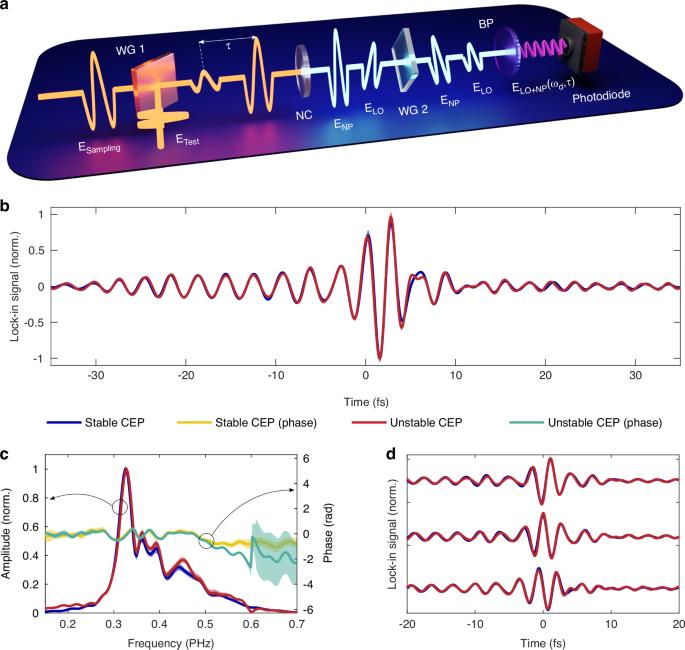
a Schematic of the optical setup. \({{\rm{E}}}_{{\rm{Sampilng}}}\) and \({{\rm{E}}}_{{\rm{Test}}}\) denote the time-varying electric fields of the sampling and test pulses, respectively. \({{\rm{E}}}_{{\rm{LO}}}\) and \({{\rm{E}}}_{{\rm{NP}}}\) represent the electric fields of the nonlinearly generated local oscillator and the nonlinearly mixed pulse. NC, WG, BP and τ refer to the nonlinear crystal, wire-grid polarizer, bandpass filter and the time delay between sampling and test pulses respectively. b, Benchmarking of the measured GHOST signals with CEP-stabilized and CEP-unstabilized pulses. c Fourier-transform spectra of the signals in (b) illustrating the frequency content with and without CEP stabilization. d Measured GHOST traces of the test pulse transmitted through glass with three slightly different thicknesses. The measurement highlights the signal’s sensitivity to the carrier-envelope phase (CEP) of the test pulse. The medium’s thickness was adjusted using a pair of fused silica wedges. The shaded areas in (b−d) correspond to one standard deviation of the measurement
Here, \({\bar{E}}_{S}\) and \({\bar{E}}_{T}\) are field strengths, \({\omega }_{S}\) and \({\omega }_{T}\) are frequencies, \({\varphi }_{S}\) and \({\varphi }_{T}\) are global phases of the sampling and test fields. The NP can be any nonlinear mixing signal30, such as sum-frequency (SFG), difference-frequency (DFG) generation, four-wave mixing (FWM), etc. By interfering the nonlinearly generated field with a “stationary” local oscillator (LO):
$${E}_{{LO}}\left(t\right)\approx {\bar{E}}_{S}^{m}{e}^{-{im}\left({\omega }_{S}t+{\varphi }_{S}\right)}$$
(4)
one can retrieve the electric field of the test pulse at each delay. The \(m\) (∈ 1, 2, …) and \(n\) (∈ 2, 3, …) factors correspond to the light-matter interaction orders used for LO and NP, respectively. The LO can be simply the sampling field itself (m = 1) or a nonlinearly generated light, e.g. second (m = 2), third (m = 3), or higher harmonics30. The intensity of the interference I(τ, ωD) at the detection frequency ωD is measured with a photodiode and is proportional to the electric field of the test pulse at time τ. Experimentally, \({{\rm{\omega }}}_{{\rm{D}}}={{\rm{m}}{\rm{\omega }}}_{{\rm{S}}}=\left(n-1\right){{\rm{\omega }}}_{{\rm{S}}}\pm {{\rm{\omega }}}_{{\rm{T}}}\), and is set by the bandpass filter (BP),
$${I}_{{LO}+{NP}}\left(\tau ,{\omega }_{D}\right)\approx {\bar{E}}_{S}^{m+n-1}{\bar{E}}_{T}\cos \left({\omega }_{T}\tau -(m-{n+1)\varphi }_{S}\pm {\varphi }_{T}\right)$$
(5)
As we show further, unlike electro-optic sampling where \(m=1\), \(n=2\), and previous implementations of GHOST (m = 3, n = 230, or m = 2, n = 335) balanced \(m=n\) combination provides a previously unexplored opportunity. In the unbalanced sum-frequency-like case, at each time delay \(\tau\), \({I}_{{LO}+{NP}}\approx {-\left(m-n+1\right)}({\varphi }_{S}+\Delta {\varphi }_{S})+{\varphi }_{T}+\Delta {\varphi }_{T}\) (Eq. 5). If the detection is not performed in a single-shot, unevenly amplified global phase instabilities \(\triangle {\varphi }_{S}\) and \(\triangle {\varphi }_{T}\), i.e. CEP instability, would average \({I}_{{LO}+{NP}}\) to zero. On the other hand, in the balanced case, \({I}_{{LO}+{NP}}\approx {\varphi }_{T}-{\varphi }_{S}+\triangle {\varphi }_{T}-\triangle {\varphi }_{S}\). When CEPs of the sampling and test pulses are locked, i.e. when pulses originated from the same laser, the CEP fluctuations are locked (\(\triangle {\varphi }_{S}=\triangle {\varphi }_{T}\)) and cancel each other out enabling extremely sensitive detection without the need for CEP-stable pulses.
In this scheme, \(\varphi_{S}=0\), fieldoscopic measurement with CEP-stabilized and unstabilized pulses is expected to yield identical results. To confirm this, we set up a GHOST detection based on the balanced SHG/SFG channel (\(m=n=2\)) utilizing a state-of-the-art octave-spanning (450–1000 nm), CEP-stable, sub-3 fs pulse36, which is split into two orthogonally polarized replicas—sampling and test—with a controlled time delay τ between them. After setting the field strength and the CEP of each pulse, the pulses are recombined and collinearly focused on the nonlinear medium. The test pulse was kept weak while the field strength of the sampling pulse was ~1 V/Å. We use a ∼ 12 μm thick z-cut α-quartz crystal as the nonlinear medium. The spectral response of the SHG/SFG channel covers the entire spectrum of the test pulse30, while the CEP stability of the pulses can be switched off on demand. We set the CEP of the sampling pulse to zero and perform sampling of the test electric field with CEP-stabilized and CEP-unstabilized pulses. Figure 1b, c confirms that the balanced (\(m=n\)) detection yields identical field traces whether or not the pulses are CEP-stabilized, as predicted.
To confirm that the measurement remains sensitive to the CEP of the test pulse, we vary its CEP by inserting a small amount of material using fused silica wedges (more in the Supplementary Information) and repeat the measurement. As can be seen in Fig. 1d, the change in the CEP of the test pulse is clearly captured by the measurement. We also note the enormous sensitivity of the measurement, which is typical for the heterodyne detection.
Fieldoscopy of strong (classical) coherent states
After confirming that the \(m=n\) channel provides a unique opportunity to access the electric field of light with CEP-unstabilized pulses, we test the concept directly with a laser oscillator. In this experiment we utilize commercial tabletop mode-locked Yb-based laser (Pharos, Light Conversion). In contrast to the previous measurements, which require sophisticated infrastructure for the generation of short (sub-3 fs) and intense (~0.4 mJ) few-cycle CEP-stable laser pulses at 1 kHz repetition rate, we employ a simple mode-locked laser delivering ~150 fs, CEP-unstable, ~8 nJ pulses centered at 1030 nm wavelength and with a 75 MHz repetition rate (more in the Supplementary Information). Figure 2 shows the results of the experiment demonstrating that the fieldoscopic measurement previously feasible only with sophisticated infrastructure is now possible with simple table-top lasers.

a Measured electric fields of coherent states consisting of a large number of photons. b Central part of the pulse (\(\left\langle n\right\rangle\) = 6.42 x \({10}^{6}\)) from the panel (a) showing clear electric field oscillations with high fidelity. c Benchmarking of the measured (blue dots) spectrum obtained by a Fourier transformation against a grating spectrometer (red curve). d Dependence of the measured signal (\(\bar{{\rm{S}}}\)) on the electric field strength of the test pulse. e Dependence of the measured standard deviation (σ) on the electric field strength of the test pulse. f Dependence of the measured signal (\(\bar{{\rm{S}}}\)) on the electric field strength of the sampling pulse
We study our concept in detail by measuring the electric field of the laser oscillator at various test and sampling pulse energies (Fig. 2a). For each measurement, we record a mean value of the signal and its standard deviation with a lock-in amplifier. Since our signal is expected to be proportional to the electric field, we expect a linear scaling of the mean signal with the field strength of the test pulse – that is confirmed by the experiment (Fig. 2d). On the other hand, three photons of the sampling pulse contribute to the heterodyne detection in the SHG/SFG (\(m=n=2\)) channel (Eq. 5). We conduct a similar power scaling experiment by varying the field strength of the sampling pulse while keeping the test field unchanged (Fig. 2f).
In ideal environment with only quantum noise (due to the probabilistic nature of photons) and in the absence of classical noise (eg. jitter, electrical or environmental instabilities) one expects the standard deviation of the electric field amplitude to remain constant, regardless of the number of photons in the pulse37. In our experiment however, we observe that the standard deviation of the measurement scales linearly with the test field strength (Fig. 2e). This is expected since any practical system is a subject of the classical noise. We attribute this scaling to the dominance of the classical noise over quantum in the regime of strong (classical) coherent states consisting of many photons. This suggests that in this regime, the standard deviation is primarily limited by experimental stability, rather than the probabilistic nature of the photons. However, the contribution of the classical noise is expected to decrease as the test field (i.e., the number of photons) is decreased. Conversely, quantum noise—which is inherently associated with photon statistics – becomes more pronounced as the number of photons in the pulse is decreased. Therefore, we expect the quantum noise to be dominant in the regime of weak coherent states.
Fieldoscopy of weak (quantum) coherent states
Our approach not only allows us to utilize stable table-top lasers at high 75 MHz repetition rate, but it also removes the noise associated with the CEP fluctuations and highly non-linear light-matter interaction. Additionally, in contrast to broadband few cycle pulses (Fig. 1), narrow bandwidth laser oscillator pulses allow us to utilize thick nonlinear crystal (for higher signal strength) since the phase matching restriction is drastically eased. Having these advantages, we perform electric field measurement of very weak laser pulses to enter the regime of weak coherent states where quantum properties dominate over classical. Since our laser photon energy corresponds to about 1.2 eV (1030 nm wavelength) one enters this regime at pulse energies on the order of 193 zepto joules. We attenuate the test pulse down to the zepto joule level and perform the measurement. We measure the test field scaling as in Fig. 2d but in the zepto joule regime. Surprisingly, despite the fact that the pulse energy is of zepto joules only, the sensitivity of the detection remains similar to the strong (classical) pJ-scale regime. As discussed earlier, we attribute this to the absence of the CEP noise and low-order non-linear light-matter interaction. However, stability of the table-top laser, MHz repetition rate, thick nonlinear medium and eased phase matching condition are beneficial as well.
We note that in our classical regime, the measured signal and a corresponding standard deviation scale linearly with the test field strength (Fig. 2d, e). Since we are primarily interested in the deviation from the classical regime, in Fig. 3b, c we divide the mean and the standard deviation by the test field strength (~\(\sqrt{\left\langle n\right\rangle }\)), so that in the classical regime these ratios are constant (which we further normalize to 1). Interestingly, when the mean photon number of the test pulse approaches 1 (~193 zJ), we observe a clear breakdown of the classical regime, both in the measured signal and the standard deviation. In particular, in the regime of weak coherent states, the scaling of the signal with the electric field becomes nonlinear. We note that in the classical description of electromagnetic waves, the scaling remains strictly linear regardless of the light field strength. The deviation from the linear scaling is a clear signature of the quantum nature of light, indicating that quantum properties (associated with coherence and photon statistics) become dominant and captured by our experiment.
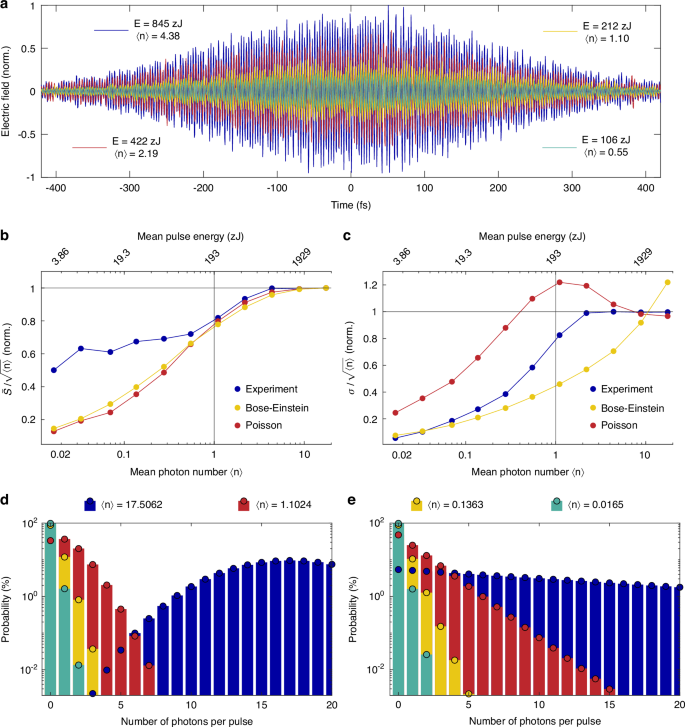
a Measured electric fields of several weak coherent states consisting of a small number of photons. b Measured and simulated breakdown of the mean signal (\(\bar{{\rm{S}}}\)) from the linear scaling. c Measured and simulated breakdown of the linear scaling of the measured standard deviation (σ). Poisson (d) and Bose-Einstein (e) probability distributions for mean photon numbers in (a)
Photon statistics analysis
Different quantum states of light are associated with unique photon statistics. In particular, coherent states follow the Poisson probability distribution, while non-coherent (thermal) light can be described by the Bose-Einstein probability distribution. We evaluate these distributions for the experimental mean photon numbers (Fig. 3d, e), with further details provided in Methods. As can be clearly seen, when the mean photon number \(\left\langle n\right\rangle\) approaches 1, the probability of the test pulse containing zero photons exponentially increases in both, Poisson, and Bose-Einstein cases.
In contrast to intensity-based measurements, direct access to the electric field serves as an observable even in cases where the test pulse contains no photons (i.e., the vacuum state). This can be intuitively understood as follows. In intensity-based measurements, reducing the photon number by half (or blocking every other pulse) would halve the detected signal. When measuring the field however, reducing photon number by half reduces the field amplitude by only ~ \(\sqrt{2}\) (since the signal ∝ electric field, which scales with the square root of intensity), which is not equivalent to blocking every other pulse (more in the Supplementary Information).
Since our measurements are conducted with a laser, we expect the experiment to mainly follow the photon statistics of coherent light described by the Poisson probability distribution. We first model our experiment (more in Methods) based on the Poisson probability distribution. Indeed, our model—where the electric field serves as an observable—predicts a deviation from the linear classical regime when the mean photon number approaches 1 and below (Fig. 3b, c). For the scaling of the mean value of the signal (Fig. 3b), our model agrees with the experiment. Surprisingly, however, the scaling of the experimental standard deviation significantly disagrees with the model. In particular, as the mean photon number approaches 1, the standard deviation is expected to increase (Fig. 3c, red curve) reaching its maximum when the mean photon number is 1. This is because for \(\left\langle n\right\rangle\) = 1 the probability of a pulses in the vacuum state is close to 50% (Fig. 3d). Overall, the power scaling of the standard deviation based on Poisson statistics exhibits a distinct peak at \(\left\langle n\right\rangle\) = 1. In our experiment however, this feature is much less pronounced, which indicates a deviation from a perfectly coherent state.
To verify that the experimental observation is indeed a signature of the deviation from coherent properties, we re-model our experiment using the Bose-Einstein probability distribution (Fig. 3b, c, yellow curve). Interestingly, we find that the scaling of the mean value of the signal follows a similar trend to that predicted by Poisson statistics. This occurs because, although the Poisson and Bose-Einstein probability distributions describe different states of light, they appear similar in the regime of weak coherent states with \(\left\langle n\right\rangle\) \(\approx\) 1 (Fig. 3b, c, green and yellow bars). However, the scaling of the standard deviation according to the Bose-Einstein probability distribution differs significantly from that of Poisson statistics (Fig. 3c, yellow curve). In particular, the standard deviation monotonically decreases as the mean photon number decreases, which is similar to our experimental observation. Overall, our experiment appears to lie between of these two extremes—perfectly coherent and perfectly thermal states.
Intrapulse coherence
The observed deviation from perfectly coherent light could potentially be attributed to the variations in the coherence across the pulse. The direct access to the electric field in our experiment allows us to perform the same analysis for different regions of the pulse—the front, center, and tail. We utilize a Gabor method where a portion of the measured mean values and standard deviations of the pulse is multiplied by a Gaussian window as shown in Fig. 4a. The results of this analysis are presented in Fig. 4b, c. Regarding the mean value of the signal, we observe a trend similar to Fig. 3b, with no significant difference in scaling between different pulse regions. However, the standard deviation analysis reveals that different parts of the pulse exhibit different photon statistics. Notably, a characteristic feature of coherent Poisson statistics is clearly observed at the regions of the pulse with low intensity. As predicted by our model (Fig. 3c), the standard deviation peaks around \(\left\langle n\right\rangle\) = 1, a hallmark signature of a coherent state described by Poisson statistics. However, this feature is much less pronounced for intense parts of the pulse. Since most of the pulse energy is concentrated in this region, the overall pulse coherence is dominated by this region. This explains why the overall pulse coherence (Fig. 3b, c) looks similar to the coherence of the most intense part of the pulse. As previously discussed, variations in intrapulse coherence are generally expected in intense mode-locked lasers.
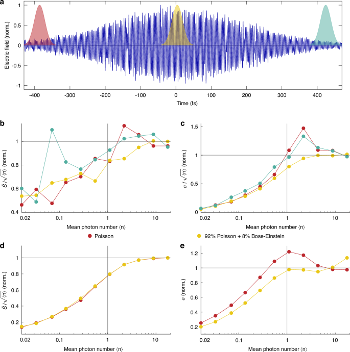
a Measured electric field of a weak coherent state (\(\left\langle n\right\rangle\) = 4.38) with corresponding Gaussian windows used for the evaluation of intrapulse photon statistics in (b) Measured breakdown of the linear scaling of the mean signal (\(\bar{{\rm{S}}}\)). c Measured breakdown of the linear scaling of the standard deviation (σ). d Simulated breakdown of the linear scaling of the mean signal (\(\bar{{\rm{S}}}\)). e Simulated breakdown of the linear scaling of the standard deviation (σ). The colors of the curves in (b, c) correspond to the Gaussian windows in (a)
Finally, we model intrapulse coherence as a time-varying combination of coherent and thermal states of light, described by the Poisson and Bose-Einstein probability distributions (Fig. 4d, e). We note a deviation from purely Poissonian statistics towards a mixed contribution of Bose–Einstein distribution, which increases with the number of photons in the pulse.