
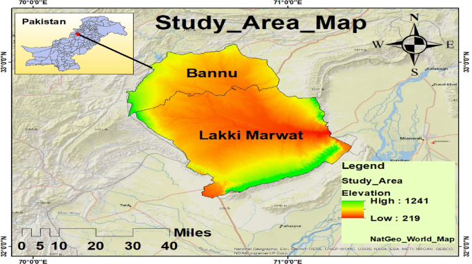
The study was carried out in the Bannu and Lakki Marwat districts of Khyber Pakhtunkhwa (KP), Pakistan’s province (Fig. 1). Both are located in a hot, semi-arid temperature zone and are connected to the Indus Flyway, which is a key crane migration path28. The 1,227 km² Bannu District is roughly 190 km south of Peshawar and is situated between latitudes 32°16′N and 33°5′N and longitudes 70°23′E and 71°16′E29. The Kurram and Gambila (Tochi) Rivers drain it, creating a basin that sustains seasonal wetlands that are essential to migratory birds28. With altitudes between 200 and 300 m, it is located close to 32.161°N, 70.191°E and is bounded by Isakhel (Punjab), Waziristan, Bannu, and Karak. With the Kurram and Tochi Rivers flowing through it and joining the Indus River, the district is made up of flat plains and outlying hills. Hot, dry summers (35–48 °C), mild winters (4–27 °C), little precipitation (290–350 mm), and frequent dust storms in May–June are characteristics of the climate. Because of their wetlands, croplands, and riverine ecosystems, both districts are important migratory crane stopping and wintering habitats, particularly for the Demoiselle Crane and Eurasian Crane18.
Data types and source
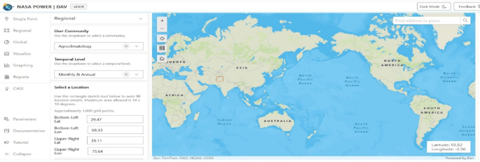
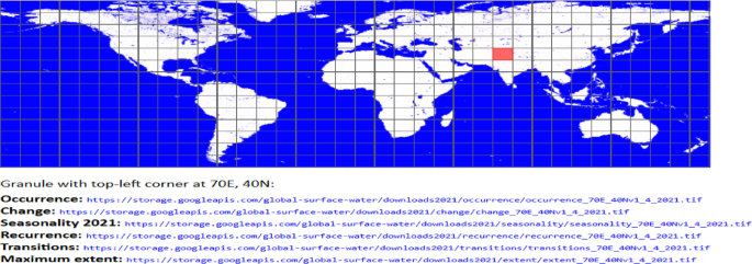
Landsat satellite images with a spatial resolution of 30 m were acquired for the years 1994 to 2024 from the U.S. Geological Survey (USGS) [https://www.usgs.gov/] and downloaded via Google Earth Engine (GEE) for further analysis. With the accumulation of large volume satellite images and the advancement of cloud computing technology, Google Earth Engine (GEE), a cloud computing platform specialized in processing geospatial data, has been increasingly applied for monitoring large-scale land cover/land use change31,32. To ensure high-quality data and minimize cloud interference, scenes with cloud cover less than 10% were selected. The imagery was obtained from Landsat Collection 2 Level-2 products, specifically: Landsat 4–5 TM C2 L2 for 1994, Landsat 7 ETM+ C2 L2 for 2004 and Landsat 8–9 OLI/TIRS C2 L2 for 2014 and 2024. Detailed metadata on acquisition dates, image dimensions, and sensor types is provided in Table 1. Daily temperature and precipitation data (1984–2024) were retrieved from the NASA (National Aeronautics and Space Administration) Langley Research Center (LaRC) Prediction of Worldwide Energy Resources (POWER) project funded through the NASA Earth Science/Applied Science Program [https://power.larc.nasa.gov/data-access-viewer/] as shown in Fig. 232. Additionally, Global Surface Water datasets (March 1984 to December 2021) were downloaded from the Global Surface Water Data Access Portal [https://global-surface-water.appspot.com/download]33. These datasets, including occurrence, change, seasonality, recurrence, transitions, and maximum extent, are freely available and provided as tiled GeoTIFF files at a 10° × 10° spatial extent, as depicted in Fig. 3. Users can select and download individual datasets by clicking on specific tiles from the interactive global map interface.
The land surface flow in the study area.
Data pre-processing
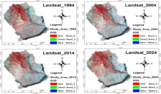
Landsat composite images (1994–2024), as shown in Fig. 4, were generated using Google Earth Engine (GEE). A shapefile representing the study area (Bannu and Lakki Marwat districts) was uploaded to GEE and used to clip Landsat imagery to the defined extent. Cloud-free composite images were created by applying filters (cloud cover < 10%) and using the median reducer to generate annual or seasonal composites from Landsat Collection 2 Level-2 Surface Reflectance data. The composite images were then exported from GEE and processed in ArcGIS. Using the Layer Stacking tool, the spectral bands were organized for visualization and analysis. Although the data were already radiometrically and geometrically corrected by USGS, further geometric alignment was ensured using the Resampling tool to maintain spatial consistency across years. The final study area was delineated using the same shape file, and each composite was clipped using the Extract by Mask tool in ArcGIS to restrict analysis to the defined region.
Landsat satellite images for the years 1994, 2004, 2014, and 2024.
Ecological habitat criteria for cranes
To enhance the ecological validity of the geospatial analysis, habitat suitability factors for Demoiselle and Eurasian cranes were identified using published ecological requirements. Both Demoiselle and Eurasian cranes are known to prefer open vegetation, shallow water areas (< 30 cm), low disturbance habitats, and extensive roosting sites in proximity to agricultural areas and seasonal wetlands. In this study, higher NDVI values were considered to represent suitable vegetation, while NDWI, MNDWI, and LSWI values were used to determine shallow water availability, which is important for roosting and foraging. LULC categories were associated with ecological processes, where croplands and wetlands were considered foraging grounds, riverine areas were considered migratory stopovers, and urban areas represented disturbed areas. Because there were no data on species presence at a fine scale, a proxy-based suitability assessment was used, which is a limitation.
Land use land cover (LULC) classification and change detection
A supervised classification approach was used to map Land Use Land Cover (LULC) across the study area, following the methodology of Ullah, Ullah34. Landsat satellite images (1994–2024), acquired via Google Earth Engine and processed in ArcGIS 10.5, were first subjected to radiometric and geometric corrections, including atmospheric correction36,37, to ensure accurate temporal comparisons. Multispectral band stacking and image resampling were performed to enhance the quality of classification. The LULC classification was conducted using multi-temporal datasets to identify and quantify land cover changes between years. Five major LULC categories were defined: Barren Land, Built-up Area, Crop Land, Trees, and Water Body. The classification of land use/land cover was done using the Maximum Likelihood (ML) supervised classification technique, which was chosen based on its ability to handle multispectral Landsat data effectively. The training samples were chosen using a combination of high-resolution Google Earth images, field validation, and existing land cover maps. For each LULC category, 50 to 60 polygons were delineated, representing a range of ecological conditions and spatial distribution, resulting in 250 to 300 training samples per year. Change detection analysis was conducted on a pixel-by-pixel basis to calculate the rate of change (hectares/year) across different land cover classes. Cross-tabulation analysis using the Tabulate Area tool in ArcGIS 10.5 was performed to examine the quantitative conversions among LULC categories38,39,40. Classification accuracy was assessed through 100 ground-truth points based on visual interpretation of high-resolution imagery from Google Earth. Coordinates for validation were referenced from both direct observation and literature. Change detection between 1994 and 2024 was further performed by subtracting pixel values of classified images, with threshold values applied to highlight significant transitions. A final change detection map was generated, and post-classification comparison methods were considered to improve the robustness of the results.
Google earth interpretations
In this study, Google Earth was utilized to access historical high-resolution imagery to support land use and land cover (LULC) change detection. The time slider tool in Google Earth allowed for visual inspection of imagery from the years 1984, 1994, 2004, and 2024, enabling decadal comparisons. These images were carefully examined to identify major transitions in land cover types, such as the expansion of built-up areas, reduction in vegetation cover, and changes in water bodies. This visual assessment served as a valuable supplementary method to validate the classification outputs and helped enhance the interpretation of spatial and temporal landscape changes within the crane habitat areas.
Accuracy assessment using confusion matrix and google earth validation
To ensure the reliability of the land use/land cover (LULC) classification, an accuracy assessment was performed using the confusion matrix approach in ArcGIS 10.541,42. The accuracy of classification was evaluated independently for 1994, 2004, 2014, and 2024 on ≥ 100 randomly validation points per year. The confusion matrix, Overall Accuracy (OA), User’s Accuracy (UA), Producer’s Accuracy (PA), and Kappa statistic were calculated for each year. A combined accuracy test is also presented for comparison. A total of 100 random reference points were generated and visually verified using high-resolution imagery from Google Earth. The classified land cover types were compared against these ground-truth points to calculate standard classification accuracy metrics (Table 2). The results indicate an Overall Accuracy of 96%, demonstrating a high level of agreement between the classified map and the reference data. The Kappa coefficient was 0.93, suggesting excellent classification performance beyond random chance (Table 3). Class-wise User’s Accuracy ranged from 75% (Trees) to 100% (Built-up Area, Crop Land, and Trees), while Producer’s Accuracy ranged from 75% (Trees) to 100% (Crop Land). This assessment confirms the robustness of the LULC classification and validates the reliability of the derived land cover maps for further spatial analysis in this study.
Kappa coefficient (K̂)
Measures agreement between classified and reference data while correcting for chance agreement:
$$K=\frac{\text{P}\text{}\text{o}-Pe}{1-Pe}$$
Where Po is the percentage of cases correctly classified (i.e., total accuracy) and Pe is the projected percentage of cases correctly classified by chance. Even though K can have a magnitude between − 1 and + 1, only positive values are often significant because negative values can be difficult to understand and indicate a level of agreement that is lower than that because of chance43. The greatest value of perfect agreement is + 1, and the value is 0 when the observed agreement is equal to the amount brought about by chance43. It is common to interpret the magnitude of the kappa coefficient in terms of a scale. Remote sensing applications have made considerable use of the interpretation scale proposed by Landis and Koch45.
Overall accuracy (OA)
Reflects how reliable the classification is for users (sensitive to commission error):
$$OA=\frac{\sum\text{X}\text{i}\text{i}}{N}$$
X 100.
Whereas Xii is the number of correctly classified samples for class i (diagonal elements) and N is the total number of reference (ground truth) samples.
Indices calculation
Three important remote sensing indices, the Normalized Difference Vegetation Index (NDVI), Normalized Difference Water Index (NDWI), and Land Surface Water Index (LSWI), were computed from Landsat imagery using ArcGIS software to evaluate the environmental factors affecting the habitat suitability of migratory crane species, particularly the Demoiselle Crane and Eurasian Crane. In order to help identify appropriate stopover and wintering sites for crane conservation planning, these indices collectively provided a thorough evaluation of the seasonal and geographical variations in habitat conditions throughout the research area45.
Normalized difference vegetation index (NDVI)
One of the most used vegetation indicators for tracking the health and amount of greenery worldwide is the NDVI46. Because of the existence of chlorophyll, healthy vegetation absorbs a large percentage of the visible electromagnetic spectrum, particularly blue light (0.4–0.5 μm) and red light (0.6–0.7 μm), while reflecting green light (0.5–0.6 μm)48. This is why vegetation appears green to the human eye. Furthermore, because of the interior structure of the leaves, healthy plant canopies show considerable reflectance in the near-infrared (NIR) range (0.7–1.3 μm). The NDVI is based on this difference between red light absorption and high NIR reflectance, and it is computed as:
$$NDVI=\frac{NIR-RED}{NIR+RED}$$
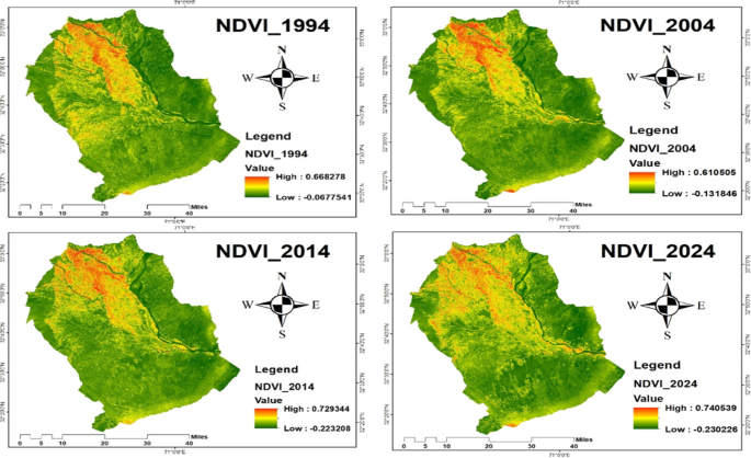
Denser and healthier vegetation is indicated by higher NDVI readings, which range from − 1 to + 1. Water bodies are typically indicated by NDVI values between − 1 and 0; barren areas, such as rocks, sand, or snow, are represented by −0.1 to 0.1; shrubs, grasses, or senescing crops are indicated by 0.2 to 0.5; and dense vegetation or wooded areas are indicated by 0.6 to 1.048. In order to comprehend the habitat requirements for migrating crane species, which mostly depend on green cover for foraging, breeding, and roosting during migration, the NDVI was computed (Fig. 5) using the Raster Calculator in ArcGIS 10.5.
NDVI of 1994, 2004, 2014, and 2024.
Annually NDVI time-series analysis (1994–2024)
An annual NDVI time-series analysis was carried out over the study area for the years 1994 to 2024 using Landsat 5, 7, and 8 surface reflectance images obtained through the Google Earth Engine (GEE) platform49 in order to assess long-term vegetation dynamics pertinent to crane habitat conditions. The QA_PIXEL band bitmask was used to eliminate cloud and shadow contamination, specifically masking bits 3 (cloud) and 4 (cloud shadow)51. In order to convert raw digital figures into top-of-atmosphere reflectance, surface reflectance values were calibrated using sensor-specific scaling factors (multiplying by 0.0000275 and subtracting 0.2)51. Each image’s NDVI was determined using the conventional NDVI calculation. A continuous annual NDVI time series from 1994 to 2024 was produced by generating annual median composites for each year and extracting the mean NDVI values within the research area. To make it easier to understand inter-annual variability, the annual NDVI data were displayed in tabular style rather than as charts that visualized the trends. Understanding the seasonal foraging and roosting needs of migratory cranes requires knowledge of long-term changes in vegetation greenness and habitat quality, which Table 5 offers. The mean and median variations (1994–2024) were also calculated using ArcGIS to assess their relevance to crane habitat.
Trend analysis
Temporal patterns of NDVI, temperature, and precipitation were analyzed to assess the magnitude of environmental changes and their implications for crane habitat. The Mann-Kendall trend test was employed to identify the significance of monotonic trends, and Sen’s slope estimator was employed to identify the nature and magnitude of trends during the period of interest. The significance of trends was determined at a level of p < 0.05. The data on NDVI was analyzed from 1994 to 2024, while temperature and precipitation data were analyzed from 1984 to 2024.
Normalized difference water index (NDWI)
Remote sensing photography is frequently used to identify and analyze surface water bodies using the Normalized Difference Water Index (NDWI)52. The near-infrared (NIR) and shortwave infrared (SWIR) bands are used by NDWI, which was first created by McFeeters53, to highlight water-related features in a landscape. It is computed as:
$$NDWI=\frac{NIR-SWIR}{NIR+SWIR}$$
However, because both NIR and SWIR reflectance are low over open water surfaces, this variant frequently performs poorly when it comes to precisely identifying clean water bodies. In order to overcome this restriction, Xu54 suggested a modified NDWI that improves detection accuracy in turbid and built-up environments by using the green band rather than NIR. Particularly when it comes to clear or turbid water, water often has a low reflectance in the NIR and SWIR regions but a high reflectance in the blue (0.4–0.5 μm) and green (0.5–0.6 μm) portions of the electromagnetic spectrum. NDWI is a useful tool for monitoring habitat conditions for water-dependent species like migratory cranes, identifying wetland loss or gain, and contextualising changes in land cover, especially when combined with NDVI55.
Modified normalized difference water index
By substituting the green band for the Near-Infrared (NIR) band, the Modified Normalised Difference Water Index (MNDWI), put forth by Xu54, enhances the detection of water bodies and makes it more successful in differentiating water from vegetation and populated regions. The following formula is used to calculate MNDWI:
$$MNDWI=\frac{Green-SWIR}{Green+SWIR}$$
The resulting values fall between − 1 and + 1, with values above 0.5 generally denoting bodies of open water. On the other hand, vegetation shows significantly lower MNDWI values, which are frequently negative, making it possible to distinguish it from water. Low positive readings, usually between 0 and 0.2, are commonly found in built-up areas. Because of its improved spectral separation, MNDWI is especially useful for tracking water features in complex or urban landscapes. It also offers vital information about the availability of wetlands for migratory waterbirds, like cranes, which depend on surface water bodies for feeding and roosting during migration.
Land surface water index (LSWI)
A popular spectral index for identifying surface water and determining vegetation water stress in remote sensing applications is the Land Surface Water Index (LSWI)57,58. It works especially well for drought analysis, wetland mapping, and agricultural monitoring. For LSWI, the typical formula is:
$$LSWI=\frac{NIR-SWIR}{NIR+SWIR}$$
While negative readings (LSWI < 0) indicate dry soil or vegetation water stress, positive values (LSWI > 0) generally indicate high water content in plants or the presence of surface water.
Analysis of NASA power data
The temperature and precipitation data, obtained from the NASA POWER database (Fig. 2) in NetCDF format, were analyzed using ArcGIS 10.5. The NetCDF files were first converted into raster layers using the “Make NetCDF Raster Layer” tool available in the Arc Toolbox59. This process generated multi-band outputs (Red, Green, Blue), which were then exported for further analysis. Precipitation data were processed using the “Cell Statistics” tool from the Spatial Analyst toolbox to compute average precipitation across the study period59. All raster datasets were subsequently projected using the “Project Raster” tool (Data Management Tools) to convert from GCS_WGS_1984 to WGS_1984 UTM Zone 43 N. To enhance the spatial resolution of the raster layers, each raster was converted to a point feature using the “Raster to Point” tool. This conversion assigned a specific value to each cell, stored in the “Grid Code” attribute field. The Inverse Distance Weighted (IDW) interpolation method was then applied using the Grid Code field to estimate continuous surfaces from the point data. The IDW technique interpolates values at unsampled locations based on known values from surrounding points61. Despite the availability of NASA POWER temperature and precipitation data in the form of gridded raster’s, IDW interpolation was used to create continuous surfaces that are spatially consistent with Landsat raster layers. The raster layers were then clipped to the study area using the “Extract by Mask” function in ArcGIS 10.5. This is helpful for combining climate data with remote sensing data without losing the original spatial and temporal patterns. After interpolation, the study area was clipped using the “Extract by Mask” tool to retain only relevant data. This entire process was performed separately for precipitation (1984–1994) and temperature (1984–1994) datasets to generate high-resolution climatic surfaces for use in ecological and habitat analyses.
Analysis global surface water dataset
The Global Surface Water datasets (Fig. 6) developed by the European Commission Joint Research Centre (JRC) were downloaded and analyzed using ArcGIS 10.5. Upon importing, all datasets were reprojected using the “Project Raster” tool in Data Management Tools to ensure consistency with the coordinate system of the study area. The area of interest was extracted using the “Extract by Mask” tool to isolate the relevant region from the global dataset. Final map outputs were generated based on guidelines provided in the Global Surface Water – Data Users Guide (v4), which offers a comprehensive technical overview of each dataset, including purpose, description, data bands, and symbology. This documentation enabled the correct interpretation and visualization of the layers, such as occurrence, change, seasonality, recurrence, and maximum water extent. Much of the methodological background is drawn from the reference publication by Pekel, Cottam33, which details the remote sensing techniques and algorithms used in generating the datasets. These processed water datasets were used to assess long-term surface water dynamics and wetland conditions, providing valuable insight into seasonal habitat availability for migratory cranes.
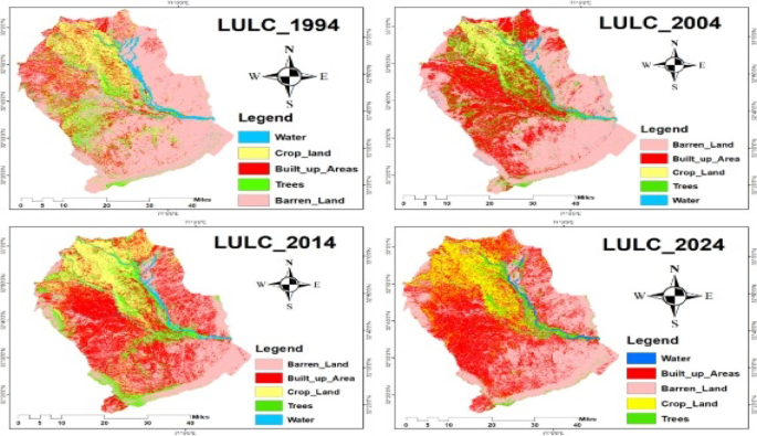
Classified Images of 1994, 2004, 2014, and 2024.