

The data is from the Norwegian Mother, Father, and Child Cohort Study (MoBa), a prospective population-based pregnancy cohort study conducted by the Norwegian Institute of Public Health. Pregnant women from across Norway were recruited between 1999 and 2008, with 41% of all pregnant women participating. The cohort includes approximately 114,500 children, 95,000 mothers, and 75,000 fathers. MoBa has been linked with Norwegian registry data provided by Statistics Norway. Version 12 of the quality-assured MoBa data files, linked with registry data collected between 1960 and 2018, was used. The current study is based on registry data for MoBa parents (n = 170,202). We gathered measures of education, income, wealth, and occupation from Statistics Norway registry data linked to the MoBa parents. The data are of high quality and not subject to attrition.
Ethics
The establishment of MoBa and initial data collection was based on a licence from the Norwegian Data Protection Agency and approval from The Regional Committees for Medical and Health Research Ethics. The MoBa cohort is now based on regulations related to the Norwegian Health Registry Act. The current study was approved by The Regional Committees for Medical and Health Research Ethics (project # 2017/2205). The project has undergone review by independent ethics advisors appointed by the European Research Council (Grant agreement No. 101045526).
Genotype quality control
Blood samples were obtained from both parents during pregnancy and from mothers and children (umbilical cord) at birth. Quality-controlled genotyping array data for the full 207,569 unique MoBa participants was recently generated65. Phasing and imputation were performed with IMPUTE4.1.2_r300.3, using the publicly available Haplotype Reference Consortium release 1.1 panel as a reference. To identify a sub-population of European-associated ancestry, PCA was performed with 1000 Genomes phase 1 after LD-pruning. The number of adults with quality-controlled genotype data used in this study is 128,310.
Measures
Four measures of SES were used: educational attainment, occupational prestige, income, and wealth. The flowchart in Fig. 6 details the data preparation process and shows the sample size used for each method and measure. The amount of missing data is the difference between the number of participants included in each method and measure and the original sample from which it was drawn.
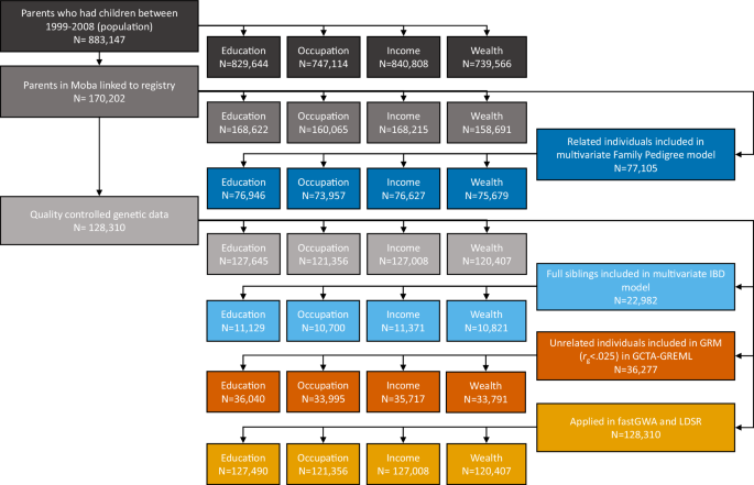
Flowchart of the population, MoBa parents, quality-controlled genetic data, the number of linked registry observations, and the sample size of each applied method.
Educational attainment
We used administrative data from the Norwegian National Educational Database, classified according to the Norwegian Standard Classification of Education (NUS2000), to identify individuals’ educational activities and backgrounds. This standard is used in Statistic Norway’s education statistics and other statistics where education is included as a variable. More information can be found at: http://www.ssb.no/en/utdanning/norwegian-standard-classification-of-education. The educational attainment data was formatted in the International Standard Classification of Education 2011 and converted to the number of years required in Norway to achieve each level. The number of years was used as it provides a more intuitive way to interpret the results and is standard in statistical genetic analyses of educational attainment. To capture the education level at a specific life stage for all participants (parenthood), we used data on the highest educational attainment recorded between ages 35 and 45.
Occupational prestige
Statistics Norway collected and coded the data on occupation. More information on data production can be found here: https://www.ssb.no/en/arbeid-og-lonn/sysselsetting. We converted the occupation codes to the international ISCO 88 format and from ISCO 88 format to Treiman’s international prestige scale (SIOPS)66. The SIOPS scale was developed through international surveys asking people to assign prestige scores to various occupations. Summarizing the results, each occupation was assigned a numeric value based on their perceived prestige. The scale ranges from 1 to 100, with higher values indicating higher perceived prestige, and the current sample includes scores from 13 to 78. This scale has been shown to be relatively stable across contexts and time points and has been widely used in social mobility research6,67,68. In addition, this occupational prestige scale correlates highly with other occupational measures both phenotypically and genetically and relates very similarly to other SES dimensions as other indicators of occupational status6,17,23.
Income and wealth
The income and wealth data we received from Statistics Norway is based on annual data from tax returns, The Tax Register, and the A-Ordning (established 2015; a digital reporting system for employers to report income and employment-related information about their employees to various government agencies). More information can be found at: http://www.ssb.no/en/inntekt-og-forbruk. An advantage of the registry data from Statistics Norway is that it is cross checked between different registries. A limitation is that income and wealth that is not reported to the various registries (i.e. tax evasion) is not included.
Due to the large distance between extreme outliers, the income and wealth data were log-transformed, after setting negative and zero values to one. Given the low number of negative values (n = 40 for income, n = 0 for wealth), this practice did not significantly affect the results. The log transformation reduces the relative distance between the observations and does so exponentially as the values get higher.
Income
We used the registry-based Statistics Norway measure of total income after taxes that consisted of wages, capital income, taxable and non-taxable transfers after taxes during a calendar year. To reduce measurement error, we averaged the income indicators across a 11-year period from age 35 to 45. We do not presume to capture the heritability of lifetime earnings.
Wealth
We used the registry-based Statistics Norway measure of gross wealth as the sum of real capital and estimated financial capital, i.e., all the financial resources a person legally has tied to their name. Again, we averaged the gross wealth across an 11-year period from age 35 to 45.
Heritability estimationFamily pedigree ACE model
The FP ACE model combines assumed genetic relatedness and measured phenotypic correlations to estimate three variance components: an additive genetic component (A), a shared environment component (C) and a residual non-shared environmental component (E)39. The pedigree structure is inferred by recorded parent-child relationships in the population data and the genetic correlations (rg) were set from to the expectation from the pedigree to be rg = 0.125 for first cousins (n = 49,423), rg = 0.5 for full siblings (n = 27,399) and dizygotic twins (n = 147), and rg = 1 for monozygotic twins (n = 136). The shared environment is assumed to be a correlation of 1 between all pairs of siblings, and 0 between first cousins in the first model. In the second model, sibling correlations are set to one, while the shared environment correlation coefficient between first cousins are free parameters to be estimated in the model. Both models included sex as a covariate.
The standardized effects of A, C, and E on the phenotype P are respectively labeled a, c, and e. The variance of the additive genetics effect (a2) equals the narrow sense heritability (h2). The equations for variance and covariance components applied in each pair of related individuals P1 and P2 are:
$${Var}(P)={a}^{2}+{c}^{2}+{e}^{2}$$
(1)
$${Cov}({P}_{1},{P}_{2})=\,{a}^{2}\times {r}_{g}+{c}^{2}\times {r}_{c}$$
(2)
Open Mx software and maximum likelihood estimation were used to estimate the a2, c2 and e2 variance components.
Identical-by-descent AE model
The IBD design applies empirical genetic correlations in a variance component model40. We estimated genome-wide identical-by-descent allele sharing (i.e., empirically derived genetic correlation) in 11,491 full sibling pairs. The sample size was not large enough to power an ACE or a sib-regression design. We, therefore, opted for an AE model with an additive genetic component (A) and a residual component (E). KING software was applied to estimate the proportion of shared alleles in each sibling pair (mean number of SNPs = 232,818, SD = 905). The models included sex as a covariate. Similarly to the family pedigree design, we applied Open Mx and maximum likelihood to estimate the A and E variance in the following equations where the genetic correlation (rg) equals the estimated proportion of genome IBD
$${Var}(P)={a}^{2}+{e}^{2}$$
(3)
$${Cov}({P}_{1},{P}_{2})=\,{a}^{2}\times {r}_{g}$$
(4)
Ultimately allowing us to calculate the heritability, as variance of the additive genetics effect (a2) equals the narrow sense heritability (h2).
GCTA-GREML
Another way to apply empirical relatedness is by comparing the genetic correlation between pairs of unrelated individuals and their phenotypic correlation. We applied genome-wide complex trait analysis (GCTA) GREML to estimate narrow sense heritability41. The standard GCTA-GREML regression model was applied,
$$y=X\beta+{Wu}+\varepsilon$$
(5)
Where β is the effect of the covariates (X), u is the effect of the standardized genotype matrix W, and ε is the residuals. The variance of y is expressed as
$${Var}(\,y)={{WW}^{\prime} u}^{2}+{I\sigma }_{{\varepsilon }^{2}}$$
(6)
The genetic relationship matrix (GRM), which is a matrix of genomic relatedness between all pairs of participants, was expressed as
$$A={WW}^{\prime} /N$$
(7)
And g was defined as a normally distributed vector of the effects of individuals with g ∼ N(0, Aσg2). Enabling us to express the variance of y as
$${Var}(y)={A\sigma }_{{g}^{2}}+{I\sigma }_{{\varepsilon }^{2}}$$
(8)
In turn allowing the calculation of heritability,
$${h}^{2}={\sigma }_{{g}^{2}}/({\sigma }_{{g}^{2}}+{\sigma }_{{\varepsilon }^{2}})$$
(9)
The GCTA software was run with restricted maximum likelihood estimation (REML), a relatedness cutoff of 0.025, a minor allele frequency (MAF) cutoff of 0.01, and covariates consisting of 20 PCs, batch, age, and sex. The number of individuals after relatedness cutoff was 36,051, and the number of SNPs after MAF cutoff was 1,235,694.
LD score regression
In addition to GREML, we applied a non-relatedness-based SNP-heritability method to estimate the total effect of common SNPs. The LD score regression approach is based on the assumption that not all causal signals are carried equally by SNPs across the genome: variants with high LD scores are more likely to carry a signal of a causal variant. In LD score regression, a reference panel is used to measure the LD of SNPs, and the extent that LD is correlated with chi square statistics from a genetic association analysis approximates the heritability of the trait in question.
To estimate LD score-based heritability, we first performed GWAS of the SES indicators. In order to include relatives in the analysis, we used the fastGWA tool in the GCTA software, which is an ultra-efficient tool for mixed linear model-based GWAS analysis69. We applied the same GRM as in the GREML analysis with a similar number of individuals and matching covariates. We included a sparse GRM matrix with relatives with an rg > 0.05 as a covariate. The number of SNPs used was 1,092,270.
We used the LD score regression software to run the LD score regression using summary statistics from the fastGWA27. The intercept represents the bias, while the slope estimates the proportion of phenotypic variance explained by both the SNPs of interest and the SNPs used to estimate the LD scores.
Assumptions of the four heritability methods
Here we present an overview of the assumptions made in the different designs with reference to a more in-depth article70.
For the FP design, it is assumed that the shared environment makes an equal contribution to the phenotype of interest across sibling and cousin pairs. If this equal environment assumption is violated, heritability estimates are likely to be inflated. We partially test this assumption by letting the cousin shared environment correlation be estimated rather than assumed. FP, as all four methods do, assumes random mating. Assortative mating can inflate heritability estimates and shared environmental effects through the reduction of phenotypic variance in the offspring through mating on similar traits71.
The IBD design relies on the assumption that the proportion of identical-by-descent segments between siblings is not affected by de novo mutations. The method also relies on the assumption that the proportion genetic correlation corresponds to genetic influences affecting the trait in question and that the additive genetic covariance corresponds to the proportion identical by descent. Breach of these assumptions may inflate or deflate the estimate, depending on the breach. Heritability estimates are likely to be inflated if shared environments are not modeled. IBD also assumes no assortative mating, which could inflate estimates.
Neither GREML nor LD score regression isolates direct genetic effects, meaning that estimates may include parental genetic effects that take effect through the environment. Indirect genetic effects are considerable for education, income, and occupational prestige22,23,48. GREML and LD score regression are also subject to a random mating assumption that might bias the estimates in either direction depending on whether the mating patterns introduce more genetic similarity, decrease phenotypic variation, or introduce environmental confounders. The GREML design assumes no gene-environment correlations, as it includes only unrelated individuals. However, confounding shared environmental effects such as population stratification would inflate heritability estimates. GREML also assumes only to capture additive genetic effects of common SNPs; exclusion of rare variants may underestimate heritability. GREML assumes that the genetic correlation derived from the GRM is true and that it corresponds to the SNP effect on the phenotype, leaving the method sensitive to cases where the SNP effects are not standardized and normally distributed or there is a strong local LD structure70.
LD score regression tackles the problem of LD in a different way, assuming that rare SNPs have larger effect sizes than common SNPs. This assumption will not hold in cases where LD scores are correlated with minor allele frequency. Another assumption is the LD reference panel. If the panel population is very different from the current population, the LD scores may not be accurate. However, genetic drift is uncorrelated with LD.
Principal component analysis
PCA is a statistical technique used to simplify complex data sets by identifying patterns and relationships between variables42. It aims to reduce the dimensionality of the data while retaining most of the variation present in the original dataset. PCA does this by transforming the original variables into a new set of variables, called PCs, which are linear combinations of the original variables.
Parallel analysis is a statistical technique used to determine the number of factors or components to retain in a PCA43. It involves comparing the eigenvalues derived from the actual data with eigenvalues derived from simulated data generated with the same number of variables and observations as the original dataset. The premise of parallel analysis is that one should retain factors or components for which the observed eigenvalues exceed the eigenvalues obtained from the random data. This method helps to avoid overestimating the number of factors or components to retain, as it provides a more stringent and objective criterion for decision-making.
We also applied the PCAtest software (https://github.com/ethanbass/PCAtest/). PCAtest is an R package designed to perform permutation-based statistical tests44. These tests assess the overall significance of a PCA, determine the significance of individual PC axes, and evaluate the contributions of each observed variable to the significant axes. 10,000 permutations and 10,000 bootstrap replicates were used to build 95% confidence intervals of the PCs. For the genetic and environmental PCAs we bootstrapped samples based on the covariance matrix and created 95% confidence intervals from 10,000 bootstrapped samples.
Reporting summary
Further information on research design is available in the Nature Portfolio Reporting Summary linked to this article.