

Tower-based observations from PLUMBER2 were utilized to validate the simulated energy and carbon fluxes. The evaluations are depicted as box plots with outliers explicitly displayed (Fig. 2b). During assessment of the entire validation set, STEMMUS-SCOPE exhibited the best performance in net radiation (Rn). The Kling–Gupta efficiency (KGE) ranged from 0.37 to 0.99, with the highest median value being 0.80 (median R², RMSE, rRMSE, and rSD values are 0.97, 38.6 W m−2, 4.09%, and 0.07, respectively). However, the performance of STEMMUS-SCOPE in the simulation of G exhibited considerable uncertainty. The KGE ranged from −15.88 to 0.58, with a median value of -3.52 (median R², RMSE, rRMSE, and rSD values are 0.22, 32.8 W m−2, 19.12%, and 1.18, respectively). The simulation of LE and H were comparable. For LE, the KGE ranged from -0.32 to 0.93, with a median value of 0.60 (median R², RMSE, rRMSE, and rSD values are 0.63, 46.2 W m−2, 7.29%, and 0.17, respectively). As for H, the KGE ranged from −1.18 to 0.90, with a median value of 0.30 (median R², RMSE, rRMSE, and rSD values are 0.68, 58.1 W m−2, 8.49%, and 0.26, respectively). The simulation of GPP is slightly more accurate than that of NEE. For GPP, the KGE ranged from -0.35 to 0.93 with a median value of 0.55 (median R², RMSE, rRMSE, and rSD values are 0.64, 3.79 µmol m−2 s−1, 6.15%, and 0.18, respectively). For NEE, the KGE ranged from −12.76 to 0.93 with a median value of −0.03 (median of R², RMSE, rRMSE, and rSD values are 0.54, 4.00 µmol m−2 s−1, 7.9%, and 0.20, respectively). The specific values are provided in Supplementary Table 6, while the detailed statistical values of each site are illustrated in Supplementary Fig. 2. We also compared the time series of observed and modelled daily LE, H, GPP, and NEE and found that the model captured annual variation of energy and carbon fluxes well (Fig. 3). Additionally, the time series of observed and modelled daily LE, H, GPP, and NEE of different vegetation type were presented in Supplementary Figs. 4 to 7. The 9 vegetation types including: SHR (Open/Closed Shrublands), CRO (Croplands), DBF (Deciduous Broadleaf Forests), EBF (Evergreen Broadleaf Forests), ENF (Evergreen Needleleaf Forests), GRA (Grasslands), MF (Mixed Forests), WET (Wetlands), and SAV (Woody Savannas). We found that STEMMUS-SCOPE slightly underestimated LE from January to June for most vegetation types except EBF. H is overestimated at DBF, ENF, and MF, and it is underestimated at WET. GPP is consistently underestimated across different vegetation types, and NEE shows significant deviations in SAV.
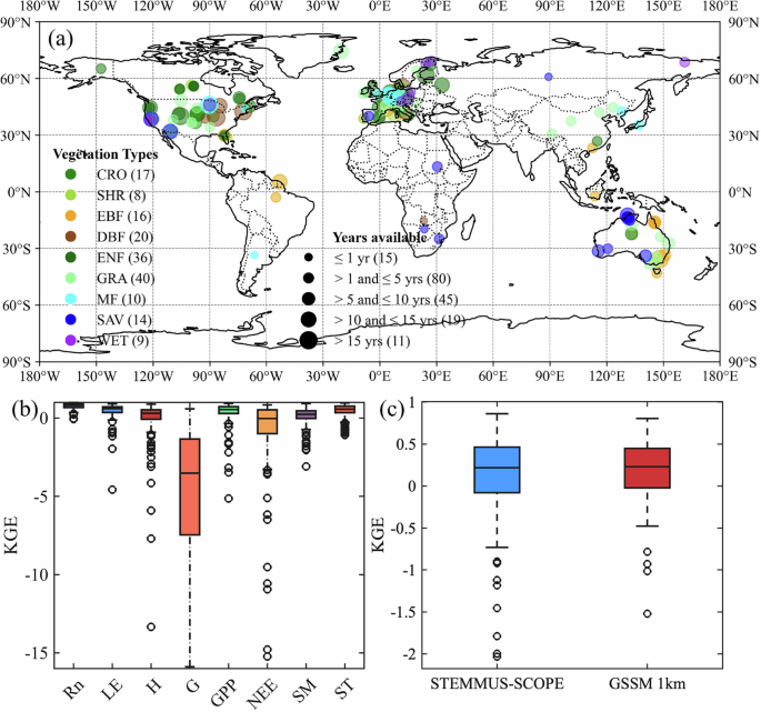
(a) Global distribution of PLUMBER2 sites; (b) Performance (Kling–Gupta efficiency, KGE) of STEMMUS-SCOPE (box plots) for the validation set of observations; (c) Performance (KGE) of STEMMUS-SCOPE and GSSM 1 km (box plots) for the validation set of observations. The box plots show (from top to bottom) the maximum, 75th percentile, median, 25th percentile, and minimum. The whiskers extend to the most extreme data points not considered outliers, and the outliers are plotted individually using the ‘○’marker symbol.
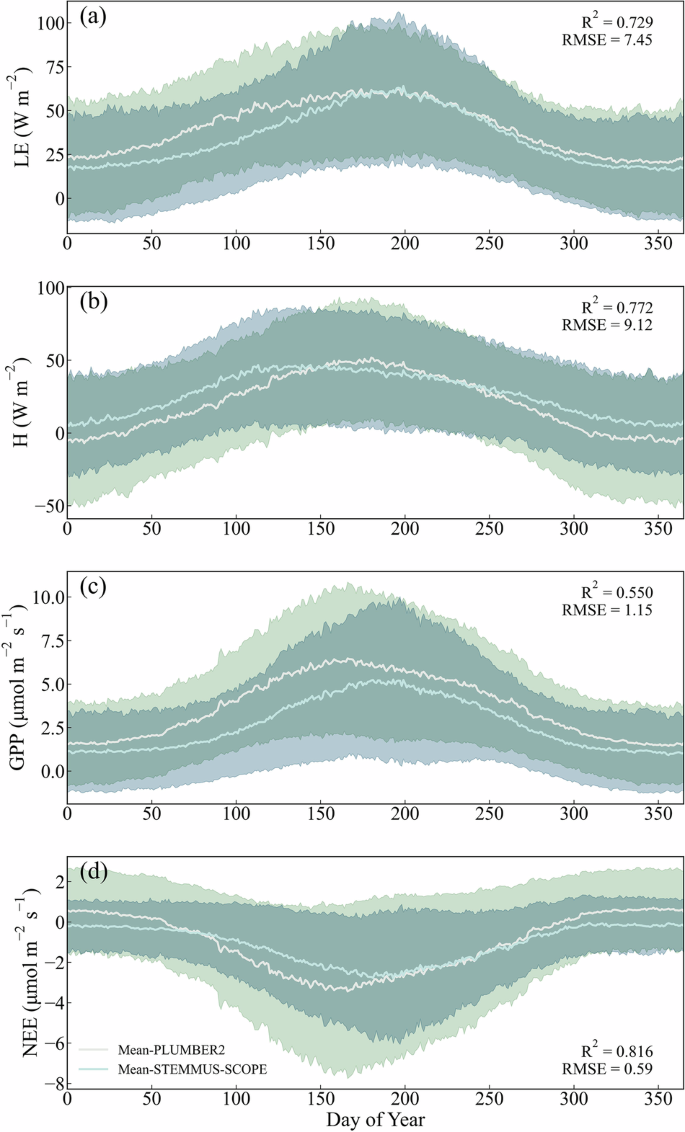
Time series of modeled and observed daily LE, H, GPP, and NEE for 170 sites.
Next, we estimated the data quality of energy and carbon fluxes at each site based on the statistical indicators. As the simulations of Rn were excellent, but those of G were unsatisfactory for most sites, these two variables were excluded in the quality classification. It should be noted that some PLUMBER2 sites lack observed G data. Furthermore, due to the absence of observation depths for G and corresponding soil moisture data at these depths, even when G observations are available, conversion to surface G is still challenging. This limitation prevents a fair comparison between observed and model-simulated G43. GPP was excluded because NEE can be directly observed, whereas GPP was derived from observed NEE. Thus, the simulations were primarily evaluated based on the KGE of LE, H, and NEE. As shown in Supplementary Table 7, out of the 170 sites evaluated, 32 sites were rated as ‘Excellent’, 64 sites as ‘Good’, 59 sites as ‘Average’, and 15 sites as ‘Poor’ for the energy and carbon fluxes.
As critical indicators of soil dynamics, the accuracy of SM and ST simulations directly reflects the reliability of other simulated fluxes. However, due to the absence of SM and ST observations in PLUMBER2, in-situ measurements from FLUXNET2015 were utilized to evaluate the accuracy and reliability of the simulations. A total of 123 sites with measurements of SM or ST were selected, as indicated in Supplementary Table 3. We compared the hourly or half-hourly in situ observations with the dataset derived from the model. For validation reliability, sites with explicit measurement depths and relatively higher-quality data were selected. As illustrated in Fig. 2b, the KGE values for SM across 96 sites varied from −0.73 to 0.93 with a median value of 0.24 (The median values of R2, RMSE, rRMSE, and rSD are 0.46, 8.84% m3 m−3, 29.11%, and 0.34, respectively). For ST, the KGE ranged from −0.31 to 0.96 with a median value of 0.56 (The median values of R², RMSE, rRMSE, and rSD are 0.88, 3.54 °C, 13.8%, and 0.39, respectively) (Supplementary Table 6). This indicates the strong capability of STEMMUS-SCOPE in tracking soil thermal and water dynamics. To further demonstrate the effectiveness of the SM simulated by STEMMUS-SCOPE, we compared it with an advanced, high-resolution global surface SM dataset (GSSM 1 km)44. Figure 2c shows that the KGE values of STEMMUS-SCOPE ranged from −0.73 to 0.86 with a median value of 0.22, which is comparable with the median value of GSSM 1 km (0.23). These indicate that STEMMUS-SCOPE is capable of capturing both surface and root zone SM dynamics. We further assessed the accuracy of SM simulation for each site.As shown in Supplementary Table 7, 38 sites were rated as ‘Excellent’, 33 sites as ‘Good’, 22 sites as ‘Average’, and 13 sites as ‘Poor’ based on the KGE value of SM at each site.
Description of the results of different vegetation types (from selected sites)
The simulations for various vegetation types were analyzed. Figure 4 demonstrates that the model accurately simulated Rn and ST for all vegetation types, consistent with the findings in Fig. 2b. Nonetheless, variations exist among the 9 vegetation types (SHR including Closed Shrublands and Open Shrublands; SAV including Savanna and Woody Savanna) regarding other output variables. The model exhibited better performance in simulating LE for forest sites, such as EBF, DBF, ENF, and MF, characterized by relatively high LAI. The model performed well in simulating H for most vegetation types except WET. The model only achieved relatively good performance in simulating G at SAV sites. Regarding GPP and NEE, the outcomes resembled those of LE due to the strong coupling between transpiration and carbon assimilation. The typical sites for each vegetation type are presented in Supplementary Figs. 8 to 16. Finally, simulations of SM were notably superior in EBF and DBF compared to other vegetation types, and the simulations of SM for two typical sites are shown in Supplementary Figs. 17 and 18.
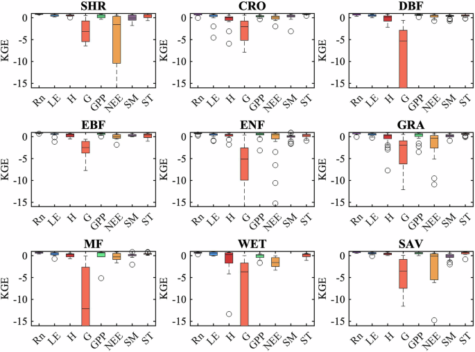
Box plots showing the Kling–Gupta efficiency (KGE) of STEMMUS-SCOPE against in-situ measurements at 9 vegetation types. On each box, the central mark indicates the median, and the bottom and top edges of the box indicate the 25th (q25) and 75th (q75) percentiles, respectively. (Note: SHR is (Open/Closed) Shrublands, CRO is Croplands, DBF is Deciduous Broadleaf Forests, EBF is Evergreen Broadleaf Forests, ENF is Evergreen Needleleaf Forests, GRA is Grasslands, MF is Mix Forests, WET is Wetland, SAV is (Woody) Savannas).
Simulation of other variables
The model also simulated SIF, reflectance spectrum, and canopy temperature, as well as their profile within canopy layers, although validating these with observations is currently challenging. Due to the time frame of this dataset spanning from 1992 to 2018, it was not feasible to validate the simulated SIF with tower-based SIF. Therefore, we compared our simulated SIF with satellite observations from OCO-2. By aligning the time periods of OCO-2 observations with our model simulations, we validated the simulated SIF at 58 stations, with most validation data concentrated between September and December 2014. For several Australian sites, validation extended through the end of 2018. To ensure compatibility with OCO-2 measurements, we computed a weighted average of the simulated SIF at 757 nm and 771 nm using the formula: (SIF757 + 1.5 × SIF771)/245. The resulting SIF values were then smoothed using a 16-day moving average to capture seasonal patterns. As illustrated in Fig. 7a, the smoothed simulated SIF closely matches OCO-2 observations, with a median R² of 0.650 and a median RMSE of 0.106 mW m−2 nm−1 sr−1. Furthermore, the model successfully captures the seasonal dynamics of SIF, as shown in Fig. 7d. To further test the reliability of simulated SIF, we also examined the correlation between modeled SIF and GPP (both observed and modeled), revealing a strong proportionality between modeled SIF and observed or modeled GPP (Fig. 5).
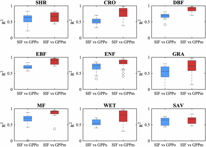
Box plots showing the coefficient of determination (R2) of modelled SIF against observed (GPPo) and modeled GPP (GPPm). The symbols are the same as in Fig. 3.
To validate the reflectance simulated by STEMMUS-SCOPE against MODIS observations, the MODIS Spectral Response Function (SRF) was applied to derive corresponding spectral bands from the model’s full-spectrum output. The simulated reflectance values were then averaged between 9:30 and 11:30 a.m.—the typical MODIS overpass time—across 8-day intervals to ensure temporal consistency. As shown in Fig. 7b and c, the agreement between simulated and observed MODIS reflectance is generally weak. For Reflectance Band 1, the median R2 is 0.19 with a median RMSE of 0.016, while for Band 2, the median R2 is 0.22 with a median RMSE of 0.010. Model performance also varies significantly across different sites. Where vegetation and soil primarily control surface reflectance, the simulated values closely align with MODIS observations (Fig. 7e). However, large discrepancies occur during periods of snow cover or extended rainfall, as expected, since the current model configuration does not account for the influence of snow, rain, or clouds on surface reflectance (Fig. 7f).
Additionally, the model simulated canopy (LEc) and soil latent heat flux (LEs), representing plant transpiration and soil evaporation, respectively. All variables of this generated physically consistent long-term dataset are listed in Table 1. To test the ability of STEMMUS-SCOPE in ET partitioning, we analyzed the simulated T/ET ratios under varying water statuses and LAI levels. As shown in Fig. 6a, the T/ET ratios increase with LAI and soil moisture. The median T/ET ratio for EBF is the highest at 0.69, and the GF-Guy site has the highest value at 0.95. The median T/ET ratio for DBF is 0.56, which is relatively high. SHR exhibits the lowest median T/ET ratio at 0.39. However, the minimum T/ET ratio is observed in the GRA (DK-Lva) at 0.07. The median T/ET ratios for other vegetation types range between 0.43 and 0.50 (Fig. 6b).
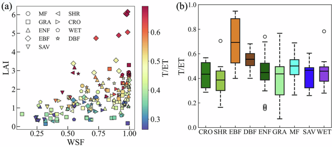
(a) Scatter plot of LAI and WSF with color-coded T/ET ratio for 170 sites with different vegetation types; (b) Boxplot of T/ET ratios for different vegetation types.
Uncertainty analysis
The novel LSMs include processes representing energy, mass, and momentum transfers in the SPAC system on a wide range of spatiotemporal scales. This inevitably results in increased model complexity to account for the interactions between the atmosphere and the land surface. The evaluations of simulated land surface fluxes, SM, and ST remain highly uncertain46,47,48,49.
The conceptual illustration of uncertainty sources in the simulations is shown in Supplementary Fig. 19. The uncertainty of the datasets produced by STEMMUS-SCOPE could be classified into four types:
-
(1)
Uncertainties in forcing data: the gap-filled meteorological data and the vegetation and soil information for running STEMMUS-SCOPE (e.g., radiation, precipitation, air temperature, wind speed, humidity, LAI, initial conditions of SM and ST);
-
(2)
Uncertainties of the parameters: the fixed default parameters used to simulate the eco-hydrological processes (e.g., Vcmax, saturated SM, saturated conductivity (Ks));
-
(3)
Uncertainties in the model structure: inaccurate representations of bio-physiological processes (e.g., ignored soil freezing-thawing processes, the 1-D nature of the model);
-
(4)
Uncertainties in the measurements used for model validation.
The uncertainties in forcing data
The proposed dataset is derived based on forcing data provided by PLUMBER2. The uncertainties that exist in the forcing data (i.e. LAI and precipitation), due to the gap-filling algorithm, will be propagated to the outputs. We next discuss uncertainties related to LAI, precipitation, land cover and vegetation properties among others.
As Supplementary Fig. 20 shows, the simulated GPP can be considerably underestimated due to the low LAI input50. To further test the uncertainty induced by LAI, we doubled the value of LAI while keeping other driving data unchanged. The results showed that the simulated values of GPP and NEE increased significantly (KGE increased from −0.24 to 0.01 for GPP, and from −1.02 to −0.58 for NEE respectively; Supplementary Figs. 20 to 22). Although there are two LAI time series in PLUMBER2 that can be used to drive LSMs, it should be noted that much uncertainty still exists in the remote sensing LAI when it is used at site scale. Such large uncertainties in remote sensing LAI products include the errors in retrieving LAI from satellite images and the mismatching between the spatial-scale of the satellite data and the site-scale fluxes51. Numerous studies have shown that LAI is a key forcing data of LSMs and it directly influences the radiative transfer and photosynthesis51,52. Especially for the sparsely vegetated areas (e.g. arid and semi-arid areas), the uncertainties in LAI result in large deviations in the simulations of GPP and LE53. Additionally, the uncertainty of LAI can significantly affect the simulation of reflectance in the SCOPE model, thereby influencing radiative transfer as well as the energy and water-carbon balance of the canopy and soil. As such, precise input LAI would be greatly valuable for constraining models. Incorporating field-measured LAI into forthcoming flux tower databases would enable bias-correction and validation of remote sensing LAI, subsequently facilitating their utilization in model forcing or direct evaluation of simulated LAI by models.
As an important forcing variable, the quality of precipitation data determines the accuracy of simulated SM which is sensitive to precipitation, especially in water-scarce areas54,55,56. Generally, sensor malfunctions or blockages in the rain bucket can lead to missing precipitation data. Subsequent gap-filling of precipitation data by global reanalysis dataset also introduces uncertainty. As Supplementary Fig. 23 shows, towards the end of the time-series, the dynamics of observed SM are not consistent with the precipitation events of the ZM-Mon site.
Determination of the vegetation type remains challenging, especially for mixed vegetation. In this study, we found that the descriptions of vegetation types for some sites were inconsistent between the driving data files and the validation data files. This discrepancy may stem from the inability to clearly delineate vegetation types for some sites. Additionally, during long-term observation experiments, certain sites underwent land use changes, which altered their vegetation types. Vegetation type determines the canopy parameters including chlorophyll content (Cab), maximum carboxylation capacity (Vcmax), dark respiration (Rd), and photosynthetic pathway (Photo_Path). Especially for the rotating cropland, the different photosynthetic type introduces large uncertainty in GPP. As we know, the water use efficiency and light use efficiency of C4 plants are higher than that of C3 plants as they have a higher light saturation point. Except for some grassland and cropland sites explicitly specified as having vegetation such as maize, switchgrass, or other C4 plants, all other sites are assumed as C3 vegetation. Analysis of two typical rotation croplands (US-Ne2 and US-Ne3: maize/soybean rotation) revealed significant inter-annual variations in observed GPP. As Supplementary Figs. 24 and 25 show, the LAI is comparable for maize and soybean; however, the observed GPP of maize is significantly higher than that of soybean. Consequently, simulations of crop rotations still exhibit significant uncertainties. In addition, the root distribution is also linked with vegetation type, such that the vegetation type could affect the root zone SM. Moreover, it should be noted that the uncertainty of LAI is greater at sites with unclear vegetation types because of the mixture of tall and short vegetation.
Finally, the uncertainty of reference height (z) and canopy height (hc) introduces significant deviations in energy flux calculations. On the one hand, the reference height (z) and hc provided by PLUMBER2 are kept constant in the model and therefore cannot realistically represent the actual conditions, especially for croplands and seasonal grasslands. On the other hand, the theory of eddy covariance requires that meteorological variables should be observed at a reference height above the canopy57, and so z is expected to be higher than hc. However, due to the lack of clarity in various site descriptions, the hc of some sites (including AU-Wrr, AU-Rob, and CN-Din sites) are higher than z in PLUMBER2, which makes it difficult for the model to converge when iterating for energy balance and results in unreasonable sensible heat flux with incorrect hc. For example, the site description for AU-Wrr states that the forests attain mature heights over 55 m and the tallest trees can reach 90 m, while the instruments are mounted at 80 m. Therefore, in the PLUMBER2 dataset, the reference height is 80 m and the canopy height is 90 m for AU-Wrr. Although we have corrected this issue during the simulation, the inconsistency between the hc provided by PLUMBER2 and the site description or the actual condition still remains significantly uncertain. This finding indicated that a physical consistent model can also be used to test the physical consistency of site data.
Canopy physiological parameters and soil property and hydraulic parameters
Whether the canopy physiological, soil physical and hydraulic parameters are adequate determines directly the performance of the model. We hypothesized that the canopy physiological parameters are relatively stable for each vegetation type, but the ignored seasonal or annual variations in these parameters may contribute to the uncertainties of the simulations. To date, with many published global datasets, such uncertainties can be further assessed. For example, the chlorophyll content (Cab) and maximum carboxylation capacity (Vcmax) are set as constants for each vegetation type, although it has been reported that these parameters may have significant seasonal and annual variabilities58,59,60. In addition, the soil hydraulic parameters could introduce uncertainty in SM simulation. For example, the saturation and residual soil water content determine the maximum and minimum values of simulated SM and the saturated hydraulic conductivity and water retention parameters of the Van Genuchten (VG) model determine the dynamics of SM. The soil parameters in this study are extracted from global datasets. Therefore, the mismatching between the grid and site scales exists and may also induce uncertainties. Specific field and lab works can be carried out to investigate specific sites, and we encourage the inclusion of the soil textures and soil hydraulic parameters in the FLUXNET site data.
Missing processes in the model structure
Although STEMMUS-SCOPE is a novel process-based LSM, it still does not contain all eco-hydrological processes. For example, processes related to freeze-thaw have been ignored which results in a large uncertainty of the SM simulation during frozen soil conditions (Supplementary Fig. 26). The user should pay attention when using the SM data at high latitude or high-altitude areas, though the vegetation is usually dormant during these periods. STEMMUS-SCOPE simulates the aggregate soil water content (sum of liquid water and frozen water), but most SM sensors only measure the liquid soil water content61,62,63. So, the model simulation in the freezing periods cannot be validated. In addition, the omission of freeze-thaw cycles and snow cover processes can introduce significant biases in reflectance simulations. For instance, at Canadian sites such as CA-NS5, the reflectance simulated by STEMMUS-SCOPE during winter is considerably lower than MODIS observations (Fig. 7(f)).
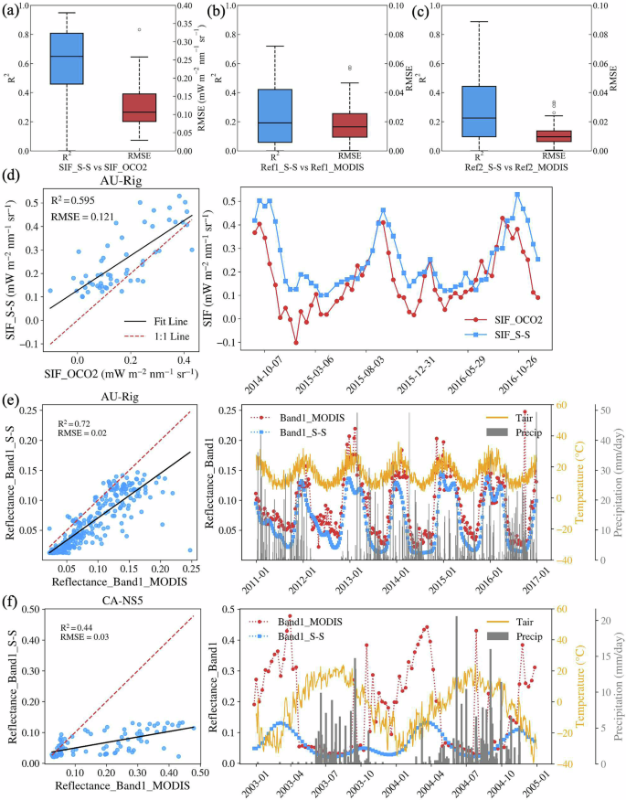
(a) Boxplot of R2 and RMSE for OCO-2 satellite SIF and modeled SIF (SIF-S-S). (b) Boxplot of R2 and RMSE for MODIS reflectance (Band 1) and modeled reflectance. (c) Boxplot of R2 and RMSE for MODIS reflectance (Band 2) and modeled reflectance. (d) Scatter plot and time series of modeled and satellite-observed SIF (OCO2) at AU-Rig site. (e,f) Scatter plots and time series of modeled and satellite-observed reflectance (MODIS) at AU-Rig and CA-NS5 site.
In addition, although the plant hydraulic module appears practical, it is relatively simple compared to those in other LSMs24,64,65,66,67,68, introducing a state-of-the-art explicit plant hydraulic scheme can further improve the performance of STEMMUS-SCOPE in arid areas. Coupling plant hydraulics in land surface models (LSMs) allows for the accurate determination of plant water potentials (root, stem, and leaf), better reflecting water stress. This approach captures the water stress responses of different plant species and improves the estimation of water, energy, and carbon fluxes68,69,70,71,72. The current version of STEMMUS-SCOPE only considers the water potential difference between the leaf and soil, while the water potential in the xylem and roots is not accounted for25. Introducing a state-of-the-art explicit plant hydraulic scheme could enhance the performance of STEMMUS-SCOPE, particularly in arid regions. The leaf water potential-based water stress factor (PHWSF) in Community Land Model Version 5.0 (CLM5) increases sensitivity to atmospheric drought compared to CLM4.569. Coupling plant hydraulics with the ED2 model allows the model to capture diverse phenologies across different plant species68. By incorporating whole plant hydraulics with water storage, the Noah-MP-PHS model captures the hydraulic behaviors of isohydric and anisohydric plants during the dry-down period70. Furthermore, the simulation of ET and GPP by VIP-PHS is significantly improved by integrating plant hydraulics into the Vegetation Interface Process model (VIP)72. Recently, an advanced plant hydraulic model incorporating xylem vulnerability has been implemented in STEMMUS-SCOPE (STEMMUS-SCOPE-PHS)71. The leaf water potential-based water stress factor (PHWSF) replaces the original soil moisture-based stress factor, better representing the impact of water stress on plant growth. The PHWSF captures the diurnal dynamics of water stress, improving the simulation of LE, NEE, and GPP. Although STEMMUS-SCOPE-PHS has been published, the advanced plant hydraulics model introduces more parameters which limits its global-scale application. Therefore, STEMMUS-SCOPE-PHS requires further validation at the PLUMBER2 sites.
Uncertainty in measurements used for validation
Uncertainties exist in the observations. Although PLUMBER2 has conducted quality control and gap-filling, some fluxes still have outliers. For example, there are many negative values in GPP due to the GPP being partitioned by the night time-based approach21,73 (Supplementary Fig. 27). In addition, the ground heat flux is not corrected to that at the soil surface which is the main reason for the low correlation between simulated and observed G. Furthermore, the measurements of SM have a large number of outliers due to the sensor failure and the measured depths that are not explained at some sites (Supplementary Fig. 28). These make it very difficult to verify the simulation of SM profiles. Since no in-situ observations are available, the validation of SIF and reflectance relies on comparisons with satellite products. However, the spatial scale mismatch between satellite observations and site-level simulations introduces inherent uncertainty into the evaluation of model performance.
To test the performance of STEMMUS-SCOPE at different levels of water status, we divide 170 sites into four groups based on their mean water stress factor (WSF, which is calculated by STEMMUS-SCOPE based on the vertical profile of root distribution and root zone soil moisture). The detailed criteria are shown in Supplementary Table 8. As shown in Fig. 8, the median KGE of LE and GPP slightly decreases with the increase of water stress, while the KGE of H increases with the increase of water stress. The reason is the strong controlling effect of radiation on LE and GPP in wet sites and while the impact of surface temperature becomes more important on H in dry sites (i.e. more radiation is partitioned to sensible heat resulting in higher surface temperature). These indicate that STEMMUS-SCOPE is capable in both wet and dry sites.
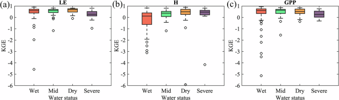
Box plots showing the Kling–Gupta efficiency (KGE) of modelled LE, H, and GPP against observed ones under different levels of water status. The symbols are the same as in Fig. 4.
Potential usage and the next step
The dataset could be used in several applications, including ecological and eco-hydrological studies, remote sensing studies, and contribute to the further development of process-based models. Furthermore, this dataset can be used to assess how changes in overall water availability across the globe influence the ability of terrestrial ecosystems to sequester carbon dioxide from the atmosphere74. The product of this study provides physically consistent fluxes data and multi-layer root zone SM and ST, based on STEMMUS-SCOPE simulations, and contributes to the understanding of terrestrial energy, water, and carbon cycles. Therefore, the SM can be used to quantify the relationship between soil water availability and eco-hydrological processes. Lastly, the dataset can be used for benchmarking various types of models, such as hydrological models, LSMs, and ESMs.
In our future work, to minimize uncertainty in the product, especially for the mixed vegetation, a vegetation growth module combined with data assimilation will be introduced into STEMMUS-SCOPE. The LAI in the current version is simply linearly interpolated from available remote sensing observations, while the actual LAI may have a higher temporal dynamics, especially for croplands. Many studies reported that combining vegetation growth model with remote sensing LAI using data assimilation methods improved the simulation of LAI as well as other vegetation growth processes75. To improve the quality of simulations for arid areas, further improvement in the plant hydraulics module is also needed. Upon the improvement in simulating plant hydraulics, the simulated plant transpiration and soil evaporation may be validated with SAPFLUXNET76. After such improvements, a global simulation can be conducted using re-analysis products as the forcing data and using International Soil Moisture Network (ISMN)77 and different global products of GPP78,79,80 and ET81,82 to validate the simulation. In addition, global satellite SM products, such as those from AMSR-E, SMOS-IC, and SMAP83,84, could also be used to validate the simulated global SM by STEMMUS-SCOPE.