

Figure 4 presents the monthly mean air temperature and cumulative precipitation recorded at the urban experimental site (TURB), along with the climatological normals for the period \(1991-2020\) from the INMET (National Institute of Meteorology) database. Temperature values were measured at \(9 \, m\) (the lowest level) above the ground at TURB. The period from January to April is notable for its higher monthly precipitation totals, with a maximum value recorded in April \((328.6 \, mm)\). Additionally, the precipitation values measured at TURB were quite similar to the climatological average. In contrast, June, July, and August showed significantly lower precipitation than the climatological average expected for this period. This substantial reduction in precipitation indicates an intense and atypical dry period.
During the wet season (months from January to April), temperatures were close to the climatological average (around \(26 \,^\circ \textrm{C}\)). This behavior suggests that during this period, climatic conditions were relatively stable, with temperatures remaining within a range near the expected average value. However, a gradual increase in temperatures was observed beginning in May, surpassing the climatological average between July and September. This period was characterized by higher temperatures than expected for the region, indicating a phase of intense warming. September was the hottest month, with maximum temperatures around \(30 \,^\circ \textrm{C}\).
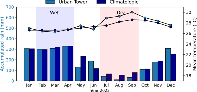
Monthly values of accumulated precipitation (bars) and average air temperature (lines) for the TURB station during 2022 (light blue) and climatological normals (dark blue) for Manaus (1991 to 2020), based on data from the National Institute of Meteorology (INMET).
In Fig. 5a, it can be observed that during the wet season, the predominant wind direction is NE (\(11.4\%\)) and E (\(9.2\%\)) with wind speeds ranging from 1 to \(4.9 \,\textrm{ms}^{-1}\), and to a lesser extent from the N. In the dry season (Fig. 5b), the NE and SE prevail, both in terms of magnitude (with speeds ranging from 1 to \(5.7 \,\textrm{ms}^{-1}\)) and frequency (\(>8\%\)). Stronger winds \((>4.1\,\textrm{ms}^{-1})\) of S and SW are also observed.
To analyze the contribution of different areas surrounding TURB to the turbulent fluxes, a footprint estimation was conducted, according to Kljun et al.70. The probability density function, which describes the upwind distance for the \(90\%\) flux contribution, reveals notable differences based on wind direction between the wet and dry seasons (Fig. 5c and d). During the wet season, the distance is greater in the E and NE directions, ranging from 400 to \(430 \, \textrm{m}\). In the dry season, the mean distance for \(90\%\) contribution in the predominant wind direction is approximately \(500\, \textrm{m}\), with significant contributions from the NE, E, and SE.
Therefore, during the wet season, the primary source area for turbulent fluxes is observed in the predominant wind direction from the NE-E sector, where there is a strong presence of impermeable surfaces such as streets and residences, and secondarily in the N-NE direction, influenced by urban infrastructure, including paved areas (Fig. 1c). In the dry season, the primary source area for turbulent fluxes remains in the NE-E direction. However, the secondary source area for turbulent fluxes shifts to the SE-S sectors, where green areas contribute more significantly (Fig. 1c).
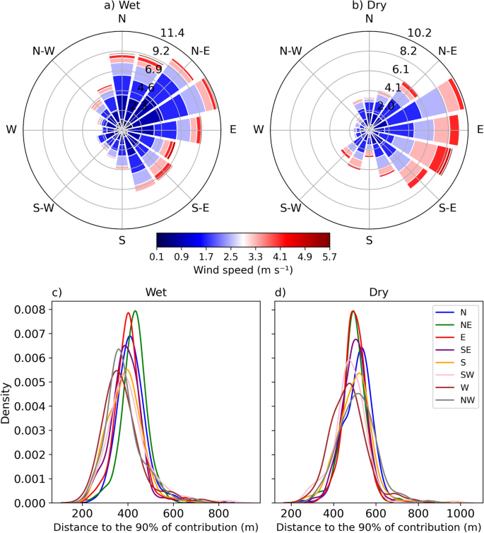
(a, b) Wind rose for the wet and dry seasons. The colors represent the average wind speed. (c, d) Probability density function of the distance of the 90% flux contribution based on wind direction for the wet and dry seasons.
Radiation fluxes
Figure 6 shows the values of shortwave (incident and reflected) and longwave radiation components (incident and emitted), and net radiation (Rn) for the wet and dry seasons in the TURB. It is evident that during the wet season (Fig. 6a), the magnitudes of \(SW_{in}\) are substantially lower compared to the dry season (Fig. 6b). This is particularly noticeable between 10:00 LT and 14:00 LT, where \(SW_{in}\) during the dry season (\(\approx 780\, \textrm{Wm}^{-2}\) at 11:00 LT) exceeds the corresponding values during the wet season (\(\approx 530 \, \textrm{Wm}^{-2}\) at 12:00 LT), with a maximum difference of \(267\, \textrm{Wm}^{-2}\) at 11:00 LT. Furthermore, the \(SW_{in}\) values during the wet season exhibited greater variability (shaded area) compared to the dry season, which can be attributed to the higher cloud cover during this period, consistent with the well-documented seasonal atmospheric dynamics of the central Amazon region71. These results shows similarities with the \(SW_{in}\) values reported by Malhi et al.27, who used data measured at the Rio Cuieiras experimental site (also named ZF2), located north in a forested area \(60 \, \textrm{km}\) from Manaus. Their study demonstrated a difference of \(166 \, \textrm{Wm}^{-2}\) between the \(SW_{in}\) values during the dry and wet seasons (from \(730 \, \textrm{Wm}^{-2}\) in the dry season to \(564 \, \textrm{Wm}^{-2}\) in the wet season at 13:00 LT, as shown in their Fig. 3). Roth et al.18 showed that in a tropical city like Singapore, the variation in \(SW_{in}\) was \(629 \, \textrm{Wm}^{-2}\) (wet season) and \(715 \, \textrm{Wm}^{-2}\) (dry season), with these values being relatively close to those found in this work. Manaus and Singapore are both cities located in the tropical region, where the presence or absence of clouds during the wet and dry seasons plays a crucial role in \(SW_{in}\) values.
Conversely, for a megacity like São Paulo, the difference in \(SW_{in}\) values measured during the wettest and driest months was only \(36 \, \textrm{Wm}^{-2}\) (Ferreira et al.72; their Table 7), indicating a less pronounced seasonal variation compared to that observed in Manaus. São Paulo does not experience as high cloud cover compared to these two cities, and therefore the variation in \(SW_{in}\) between summer and winter is smaller18,29,72.
The \(SW_{out}\) values (Fig. 6d, e) show seasonal variability similar to that of \(SW_{in}\) in terms of variation, amplitude, and anomalies, with the highest (lowest) values observed during the dry (wet) season. During the wet season, the maximum value was \(82 \, \textrm{Wm}^{-2}\) at 12:00 LT, and during the dry season, it was \(135 \, \textrm{Wm}^{-2}\) at 11:00 LT.
In Fig. 6g and h, the hourly values of incoming longwave radiation \((LW_{in})\) are shown. It is noted that \(LW_{in}\) exhibited similar maximum values during both wet and dry seasons \((\approx 442 \, \textrm{Wm}^{-2})\). During the dry season, a gradual and prolonged decline in \(LW_{in}\) was observed after the maximum, resulting in a minimum of \(410 \, \textrm{Wm}^{-2}\) at 06:00 LT. In contrast, during the wet season, the minimum value of \(LW_{in}\) was approximately \(421 \, \textrm{Wm}^{-2}\) at 04:00 LT. Therefore, during the wet season in the Amazon, \(LW_{in}\) values tend to be higher compared to the dry season29. The \(LW_{in}\) values reported by von Randow et al.29 over the Amazon rainforest ranged from approximately 400 to \(440 \, \textrm{Wm}^{-2}\) during the wet season and 390 to \(440 \, \textrm{Wm}^{-2}\) during the dry season. For a tropical city like Singapore, \(LW_{in}\) values ranged from 413 to \(445 \, \textrm{Wm}^{-2}\) and 390 to \(430 \, \textrm{Wm}^{-2}\) during the wet and dry seasons, respectively18. In a subtropical city like São Paulo, Brazil, values ranged from \(377 \, \textrm{Wm}^{-2}\) to \(436 \, \textrm{Wm}^{-2}\) for the summer (February) and from \(329-388 \, \textrm{Wm}^{-2}\) for the winter (August)72. It is observed that the \(LW_{in}\) values for Manaus are not significantly different from those observed over other sites at Amazon rainforest or in tropical regions like Singapore.
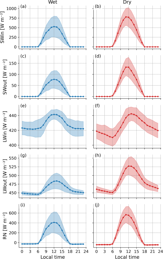
Daily variability of the radiation balance components during the wet season (blue) and dry season (red). \(SW_{in}\) and \(SW_{out}\) represent the components of incoming (a, b) and reflected (c, d) shortwave radiation, respectively. The components of longwave radiation emitted by the atmosphere and surface are represented by \(LW_{in}\) (e, f) and \(LW_{out}\) (g, h). And (i, j) net radiation \((RN = SW_{in} – SW_{out} + LW_{in} – LW_{out})\).
The \(LW_{out}\) values (Figs. 6j,k) were considerably lower during the wet season (ranging from 445 to \(484 \, \textrm{Wm}^{-2}\)) compared to the dry season (ranging from 451 to \(527 \, \textrm{Wm}^{-2}\)). This result was expected since the warmer surface during the dry season will emit a higher longwave radiation flux. The maximum difference in \(LW_{out}\) values between the seasons was \(40 \, \textrm{Wm}^{-2}\), occurring between 11:00 LT and 13:00 LT (Fig. 6l). The \(LW_{out}\) (max) values found for the Amazon rainforest, Singapore, and São Paulo were: \(426-475 \, \textrm{Wm}^{-2}\) (wet) and \(428-475 \, \textrm{Wm}^{-2}\) (dry), \(444-499 \, \textrm{Wm}^{-2}\) (wet) and \(455-511 \, \textrm{Wm}^{-2}\) (dry), and \(400-497 \, \textrm{Wm}^{-2}\) (August) and \(455-511 \, \textrm{Wm}^{-2}\) (February), respectively18,29,72. It is noted that the \(LW_{out}\) values for the city of Manaus were much closer to those of Singapore and São Paulo than to those observed over the Amazon rainforest, especially during the dry season. This indicates that the heat absorption dynamics in the urban canopy differs from those observed in the forest canopy. In the urban landscape, the three-dimensional geometry allows for multiple reflections of incident radiation, leading to a significant increase in the capture and absorption of energy by the surface. Additionally, heat conduction and convection processes play a crucial role, significantly contributing to higher longwave radiation emission from the urban surface.
The maximum net radiation (Rn) values in Manaus were 410 and \(565 \, \textrm{Wm}^{-2}\) during the wet and dry seasons, respectively (Figs. 6i-j). The lower Rn values during the wet season are often attributed to the higher cloud cover, which reduces \(SW_{in}\) in this period. However, when comparing the Rn values found here with those measured above the Amazon rainforest (\(556 \, \textrm{Wm}^{-2}\) in the wet and \(623 \, \textrm{Wm}^{-2}\) in the dry season), Singapore (\(473 \, \textrm{Wm}^{-2}\) in the wet and \(527 \, \textrm{Wm}^{-2}\) in the dry season), and São Paulo (\(452 \, \textrm{Wm}^{-2}\) in August and \(520 \, \textrm{Wm}^{-2}\) in February), we observe that the values for Manaus were considerably lower than those measured over the Amazon rainforest. This discrepancy is likely due to the relatively higher \(LW_{out}\) values in urban areas compared to forested regions.
The average albedo values (Fig. 7), which represent the ratio of \(SW_{out}\) to \(SW_{in}\), ranged from 0.15 to 0.18 for the wet and dry seasons, respectively. There are no previous reports on the seasonal variation of surface albedo in urban areas of the Amazon. The albedo values found for the metropolitan region of Manaus were higher than those (0.13) measured over the Amazon rainforest29. The values observed here are consistent with typical values reported in the literature for urban and suburban areas in other regions located at mid-latitudes (mean albedos of 0.14 and 0.15, respectively)73. These values also resemble those observed under seasonal conditions in a tropical city like Singapore, which were approximately 0.15 and 0.17 for wet and dry conditions, respectively18.
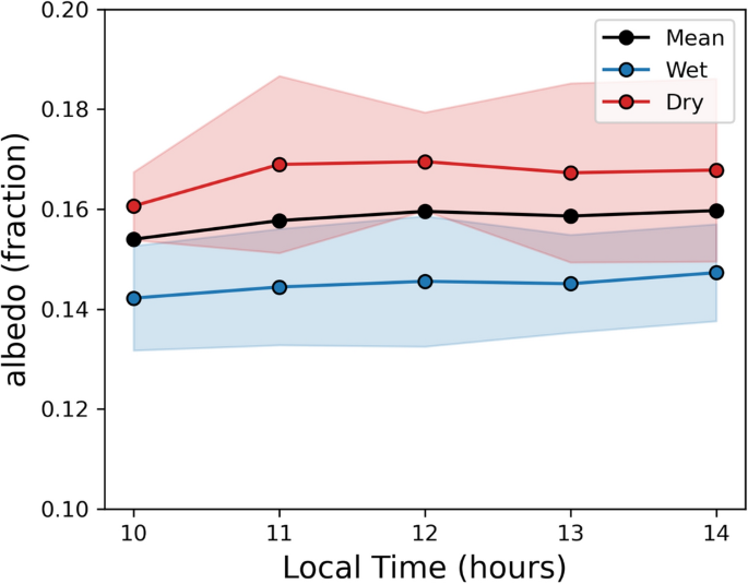
Diurnal variability (10:00 LT to 14:00 LT) of the albedo for the overall mean (black), wet season (blue), and dry season (red), measured at the urban tower in the city of Manaus.
Based on the results of the Student’s t-test (t-statistic of \(-24.34\) and p-value = 0), we can conclude that the albedo during the wet season was significantly different from the albedo during the dry season. The negative t-statistic suggests that the mean albedo during the wet season is significantly lower than the mean albedo during the dry season. Furthermore, the p-value being approximately zero indicates that the probability of observing such a large or greater difference in albedo between the two seasons, under the assumption that there is no real difference, is virtually nil. Therefore, surface reflectivity varies significantly between the wet and dry seasons.
Components of energy balance
The components of the energy balance, such as the turbulent fluxes of sensible heat (H) and latent heat (LE), as well as soil heat flux (G), for both the wet and dry seasons, are shown in Fig. 8. H values remained positive during both day and night (Figs. 8a–b), with higher values observed during the dry season, reaching a maximum of \(251 \, \textrm{Wm}^{-2}\), compared to \(119 \, \textrm{Wm}^{-2}\) in the wet season, both occurring at 12:00 LT. The minimum values were recorded at 06:00 LT during the wet season \((0.53 \, \textrm{Wm}^{-2})\) and at 05:00 LT during the dry season \((3.60 \, \textrm{Wm}^{-2})\). The differences were more significant during the daytime (Fig. 8c), where H was at least 100% higher \((>100 \, \textrm{Wm}^{-2})\) during the dry season between 10:00 LT and 13:00 LT.
Sensible heat flux remained positive even after Rn had changed sign during the night, exhibiting a distinct dynamic compared to forested regions. In urban areas like Singapore18, H stays positive after sunset, becoming slightly negative between 05:00 LT and 06:00 LT. According to Oke et al.62, there is a direct relationship between the magnitude of nocturnal positive H and urban built density. This relationship is evident in high-density cities such as Tokyo, Japan; Basel, Switzerland; Marseille, France; and Mexico City, Mexico, which are characterized by local climate zones (LCZ) classified as “compact midrise” and “lowrise” (LCZ 2 and LCZ 3). In these cities, nocturnal H remains positive, with average values ranging between \(5 \, \textrm{Wm}^{-2}\) and \(30 \, \textrm{Wm}^{-2}\) from 21:00 LT to 03:00 LT62. Conversely, in suburban area from São Paulo, H is relatively small at night, becoming negative approximately one hour after Rn turns negative and remaining so until sunrise17.
In the Amazon rainforest, H values are negative during the night27,29. However, during the day, the H values observed in Manaus were similar to those recorded in the Jaru Biological Reserve (Rebio-Jaru), located in the southwestern Amazon, with maximum values of \(117 \, \textrm{Wm}^{-2}\)29. During the dry season, H values in Manaus reached a maximum of \(250 \, \textrm{Wm}^{-2}\), exceeding those reported for Rebio-Jaru (maximum of \(180 \, \textrm{Wm}^{-2}\))29 and approaching values observed in Singapore \((226 \, \textrm{Wm}^{-2})\)18.
The behavior of LE (Figs. 8d, e) was similar in both seasons, with a decline after reaching its peak: \(132 \, \textrm{Wm}^{-2}\) at 12:00 LT during the wet season and \(121 \, \textrm{Wm}^{-2}\) at 11:00 LT during the dry season. Between 12:00 and 17:00 LT, LE values were higher in the wet season, with a maximum difference of approximately \(20 \, \textrm{Wm}^{-2}\) (Figure 8f). In contrast, during the other hours of the day, LE values were higher in the dry season, although the difference did not exceed \(10 \, \textrm{Wm}^{-2}\). Despite seasonal variations and the decrease in rainfall volume and frequency during the dry season, LE in Manaus does not appear to be significantly affected by this reduction in rainfall. This indicates that other factors and processes may play a role in influencing LE values in the urban area of Manaus.
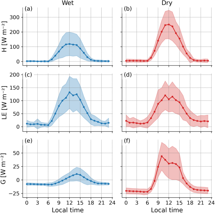
Mean diurnal variation of the components of turbulent sensible heat flux – H (a, b), latent heat flux – LE (c, d), and soil heat flux (e, f) during the wet season (blue) and dry season (red). The shaded areas correspond to the statistical error of the mean.
The LE values reported by von Randow et al.29 for the Amazon rainforest (Rebio-Jaru) were higher than those observed in Manaus, with maximum values reaching approximately \(400 \, \textrm{Wm}^{-2}\). This outcome aligns with the well-documented high evapotranspiration rates of the Amazon rainforest throughout the year, attributed to its soil’s greater water storage capacity. Nonetheless, a shared characteristic between Manaus and Rebio-Jarú is the weak seasonality in LE values.
In the case of Rebio-Jarú, von Randow et al.29 showed that the deep roots of trees could access water at greater depths during the dry season, maintaining their evapotranspiration rates, and thus, LE values did not show significant decreases from the dry to the wet season. In urban Manaus, it is observed that during the dry season, there is runoff coming from the SE-S-SW direction (Fig. 5), where there is greater green cover (Fig. 1c), which may explain the LE values during the dry season being similar to those observed during the wet season. Additionally, we believe that the low variability of LE between the wet and dry seasons in Manaus is related to the presence of moisture sources (large rivers), which contribute to maintaining high LE values during the dry season.
In a tropical city like Singapore, the seasonal variability of LE was also low, varying within a narrow range during the wet and dry seasons, with values of \(123 \, \textrm{Wm}^{-2}\) and \(105 \, \textrm{Wm}^{-2}\), respectively18. In a subtropical city like São Paulo, LE showed seasonal variations, with values of \(<50 \, \textrm{Wm}^{-2}\) during the dry season and approximately \(112\, \textrm{Wm}^{-2}\) during the wet season74.
G represents the variation in heat storage and release in the soil. The soil accumulates energy during the day (positive) and releases it (negative) at night, after sunset. During the wet season, G reached \(11 \, \textrm{Wm}^{-2}\) at 14:00 LT, while in the dry season, it reached \(44 \, \textrm{Wm}^{-2}\) around 10:00 LT, which is four times higher. The most pronounced hourly differences occurred between 09:00 LT and 13:00 LT, exceeding \(20 \, \textrm{Wm}^{-2}\). At night (20:00 LT to 05:00 LT), the dry season released (\(G < 0\)) on average \(13 \, \textrm{Wm}^{-2}\) more heat than the wet season (dry: \(-20.20 \, \textrm{Wm}^{-2}\) vs. wet: \(-7.32 \, \textrm{Wm}^{-2}\)). However, near sunrise and sunset, the differences between seasons became less significant, despite the wet season generally recording higher values. The increase in G during the dry season is due to lower cloud cover and, consequently, higher incident solar radiation on the surface, causing the soil to absorb and release more heat into the atmosphere.
In the forest, soil heat flux is generally low and does not show significant seasonal variation30, mainly due to the limitation of solar radiation caused by the dense forest canopy. Therefore, it is added to the heat storage term in biomass and air above the forest floor75. On the other hand, in pasture areas, heat flux is higher than in the forest and exhibits notable seasonal variations29, similar to those observed in this study.
Storage heat flux
The values of \(SHF_W\) (Fig. 9 a and b) and \(SHF_R\) (Fig. 9 c and d) showed similar variability during both dry and wet periods, although \(SHF_R\) was slightly lower. Both variables peaked around 8:00 LT, earlier than the typical peak time of sensible heat flux and latent heat flux. These earlier peaks are due to the low thermal capacity of the materials composing the roof and walls. The maximum \(SHF_W\) value was approximately \(25 \, \textrm{Wm}^{-2}\) higher during the dry season than the wet season, while the maximum \(SHF_R\) value remained nearly unchanged between the seasons.
\(SHF_R\) values became negative around 14:00 LT in both seasons, while \(SHF_W\) became negative at 16:00 LT. An explanation for this time lag in the behavior of \(SHF_R\) and \(SHF_W\) is the average heat storage/release capacity of each surface type (roof and wall) in the urban system. Large temperature gradients produce sudden changes in the rate of heat absorption and release, such as the “peak” in energy absorption during the early morning and the abrupt drop toward energy release (negative) in the early evening66. Heat release occurs faster from the roof than from the wall due to zinc’s lower thermal capacity (Table 3). Total heat storage in the urban layer (Figs. 9e, f) is predominantly influenced by the behavior of \(SHF_W\), contributing an average of \(72\%\) daily during the wet season and \(97\%\) during the dry season. The maximum S value was \(102 \, \textrm{Wm}^{-2}\) (wet season) and \(127 \, \textrm{Wm}^{-2}\) (dry season) at 08:00 LT, with a minimum at 18:00 LT (approximately \(-81 \, \textrm{Wm}^{-2}\) in the wet season and \(-102 \, \textrm{Wm}^{-2}\) in the dry season). During the wet season, the urban canopy had greater average heat accumulation, reaching approximately \(4.26 \, \textrm{Wm}^{-2}\), due to lower dissipation (minimum value). In contrast, heat absorption and release were higher during the dry season, leading to a smaller energy storage of \(2.17 \, \textrm{Wm}^{-2}\).
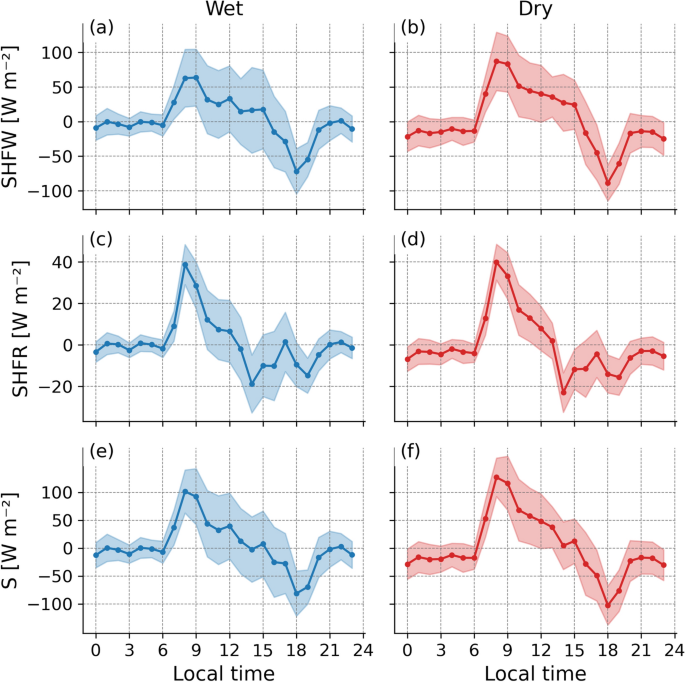
Mean daily variation of the stored heat flux in the wall – \(SHF_W\) (a, b), roof – \(SHF_R\) (c, d), and the total sum – S (e, f) for the dry (red) and wet (blue) seasons.
In forest environments, heat storage is primarily partitioned between biomass and the air above the ground75. The variability of S in the urban environment was similar to that observed in forests during the dry season30 but higher in magnitude (max: \(64 \, \textrm{Wm}^{-2}\), min: \(-32 \, \textrm{Wm}^{-2}\)), due to the different thermal properties of urban and forested surfaces. Additionally, in forests, heat storage in tree trunks accounts for about \(40\%\) of the total energy storage30. On the other hand, the maximum storage \((242 \, \textrm{Wm}^{-2})\) and maximum release \((-98 \, \textrm{Wm}^{-2})\) reported by Ferreira et al.17 were higher than the values found in this study.
Surface energy balance
The seasonal variation of the energy balance, including all convective and conductive flux components, is showed in Fig. 10. During the wet season, the H and LE exhibit similar behavior. LE plays a dominant role in energy partitioning, accounting for approximately \(46\%\) of the daily energy, while H represents \(36\%\), and G and heat stored in the canopy S contribute \(3\%\) and \(4\%\), respectively.
This pattern differs from observations in other urban regions, including tropical areas such as Singapore18, where a distinct scenario was observed. In Singapore, during the wettest period, H was \(22\%\) higher than LE and accounted for around \(52\%\) of Rn. However, in a suburban area of São Paulo, during the summer/wet season, the values were similar to those observed here for the wet season (LE was \(14\%\) higher than H, while H accounted for around \(32\%\) and LE about \(36\%\) of Rn). This observation is related to the presence of vegetation, soil moisture content, and circulation patterns influenced by sea breezes that transport moisture inland74.
Sensible heat flux dominates energy partitioning during the dry season, contributing about 55% of the total, with an average daily value of \(6.36 \, \textrm{MJm}^{-2}\textrm{d}^{-1}\). The remaining fluxes contribute 37% (LE: \(4.30 \, \textrm{MJm}^{-2}\textrm{d}^{-1}\)) and 2% (S:\(0.19 \, \textrm{MJm}^{-2}\textrm{d}^{-1}\) and G: \(-0.20 \, \textrm{MJm}^{-2}\textrm{d}^{-1}\)) to the daily average. Overall, the energy balance resembles that measured in other urban areas across various latitudes and climatic conditions. Most of the available energy at the surface during the day is transferred to the urban canopy through turbulent convection (i.e., H), evaporation from surfaces (LE: \(7.40 \, \textrm{MJm}^{-2}\textrm{d}^{-1}\)), and a smaller fraction through conduction (\(G+S\): \(5.1 \, \textrm{MJm}^{-2}\textrm{d}^{-1}\)). Thus, during this period, there is a greater accumulation of energy due to the seasonal conditions, with this energy primarily directed towards surface heating.
The H and LE observed in this study exceeded those reported in Singapore (tropical city)18 during a comparable dry season, as well as those measured in São Paulo, a large metropolitan area in southeastern Brazil17. Notably, both H and LE were also higher than the values obtained during one the first eddy covariance observations of energy fluxes in the Amazon, conducted at the Ducke Reserve in 198321 (approximately 25 km from Manaus in 1983 but now encompassed by the city). Shuttleworth et al.21 reported that LE accounted for approximately \(70\%\) of net radiation during the dry season (LE = \(8.42 \, \textrm{MJm}^{-2}\textrm{d}^{-1}\); \(Rn = 12.06 \, \textrm{MJm}^{-2}\textrm{d}^{-1}\)). In contrast, in our urban study site, LE represented only \(37\%\) of Rn (\(LE = 4.30 \, \textrm{MJm}^{-2}\textrm{d}^{-1}\); \(Rn = 11.66 \, \textrm{MJm}^{-2}\textrm{d}^{-1}\)). This substantial reduction in the proportion of energy allocated to LE was accompanied by a corresponding increase in H, which increased from \(2.85 \, \textrm{MJm}^{-2}\textrm{d}^{-1}\) \((24 \%)\) in the Ducke Reserve21 to \(6.36 \, \textrm{MJm}^{-2}\textrm{d}^{-1}\) \((55 \%)\) in our measurements. These changes are particularly relevant considering that the Ducke Reserve, once a site of primary forest, has become increasingly surrounded by Manaus’urban development76. It highlights how urbanization alters surface energy partitioning, with potential implications for urban climate.
Urban heat storage plays a significant role in energy distribution during sunrise and sunset. Together with soil heat flux, it significantly influences the heating of the urban canopy, particularly during the wet season, where S is 48% and G is 17% higher than in the dry season. During the nighttime, these contributions account for 74% and 48% of the available energy, respectively (Table 4).
The diurnal and nocturnal trends for the convective and conductive fluxes are reflected in the corresponding daily averages (Table 4). The seasonal variability of Rn and H during the daytime was similar to the daily pattern, with higher values during the dry season. In contrast, LE, G, and S showed an opposite pattern, with higher values during the wet season. However, only the nighttime seasonal behavior mirrored the daily average.
The maximum Bowen ratio \((\beta )\) during the day was observed near midday (Fig. 10c). The highest daytime values \((\approx 2.37)\) were recorded during the dry season, when H was significantly higher than during the wet season \((\approx 1.05)\). Values higher than 1 indicate that the surface directs more heat as H and are typical of dry surfaces, while values smaller than 1 indicate that LE dominates, which is characteristic of moist surfaces. The daytime results were lower than those found for Singapore (\(\beta\) values of 1.31 and 1.96 during the dry and wet seasons, respectively)18. The daily average of the Bowen ratio during the wet season (0.88) was comparable to that of São Paulo, but was lower during the dry season (1.98)74.
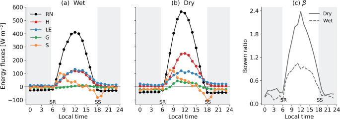
Daily variability of the hourly mean values of observed components (H, LE, and G) and estimated (S) during the wet (a) and dry (b) seasons; and Bowen ratio (c). SR – sunrise, SS – sunset.
Energy balance closure
The linear regression coefficients between the sum of energy fluxes and the energy balance, using Ordinary Least Squares (OLS) for all half-hour data in both the dry and rainy seasons, are presented in Fig. 11. The energy fluxes, \(H + LE\) (and the inclusion of the conductive terms, S and G) versus Rn exhibited relatively high values in both seasons, with a correlation coefficient \((R^2)\) varying from 0.78 to 0.87. In the rainy season, when G is included (i.e., \(H + LE + G\)), the energy balance closure was approximately 0.53 (\(R^2 = 0.81\), Fig. 11a). When S is included (i.e., \(H + LE + S\)), the correlation slightly decreases (\(R^2 = 0.78\), Fig. 11b), but there was an improvement in energy balance closure (slope \(= 0.63\)). Including both G and S resulted in a significant improvement in the correlation between Rn and the sum of the fluxes (\(R^2 = 0.80\), Fig. 11c), and in the energy balance closure (slope \(= 0.66\)). Despite the slight decrease in \(R^2\), the inclusion of S contributed to a better closure of the energy balance, reducing the imbalance between incoming and outgoing energy. The improvement in energy balance closure was more pronounced during the dry season (Fig. 11d, e, f). The \(R^2\) value was 0.84 when only G was considered, and increased to 0.87 with the inclusion of \(G+S\) (Fig. 11f). The slope increased from 0.63 with G to 0.80 with \(G+S\).
The residual average energy balance decreased (Table 5) from \(37.51 \, \textrm{Wm}^{-2}\) (G) to \(25.46 \, \textrm{Wm}^{-2}\) \((G+S)\) in the wet season and from \(20.77\, \textrm{Wm}^{-2}\) (G) to \(15.46 \, \textrm{Wm}^{-2}\) \((G+S)\) in the dry season. Additionally, RMSE values were significantly reduced from \(120.61 \, \textrm{Wm}^{-2}\) to \(104.97 \, \textrm{Wm}^{-2}\) in the wet season and from \(112.33 \, \textrm{Wm}^{-2}\) to \(90.92 \, \textrm{Wm}^{-2}\) in the dry season, indicating improved prediction accuracy when both components \((G+S)\) were incorporated into the model (Table 5).
The slope values (ranging from 0.53 to 0.80) and \(R^2\) coefficients were within the ranges identified in 22 FLUXNET network sites69, where slopes varied from 0.53 to 0.99, and \(R^2\) from 0.64 to 0.96. With the inclusion of \(G+S\), energy balance closure exceeded the average slope of 0.79 reported by Wilson et al.69, as well as values for São Paulo (0.79 in February and 0.75 in August)74. Furthermore, incorporating \(G+S\) improved the statistical metrics, suggesting that the S variable plays a critical role in energy balance closure, consistent with findings in the Amazon rainforest30, where a reduction in imbalance and an improvement in energy balance closure (wet: 0.94 and dry: 0.89) were observed with the inclusion of canopy heat storage.
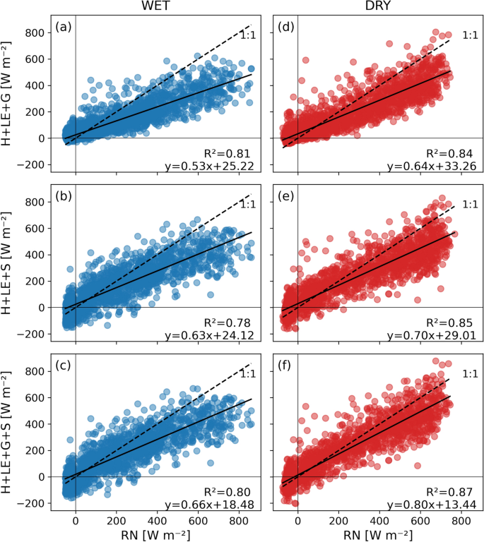
Linear regressions between the sum of energy fluxes \(H + LE + G\) and net radiation Rn (a, d); considering the inclusion of \(+S\) (b, e); and the incorporation of all terms \(G + S\) (c, f), for the wet (blue) and dry (red) seasons.