

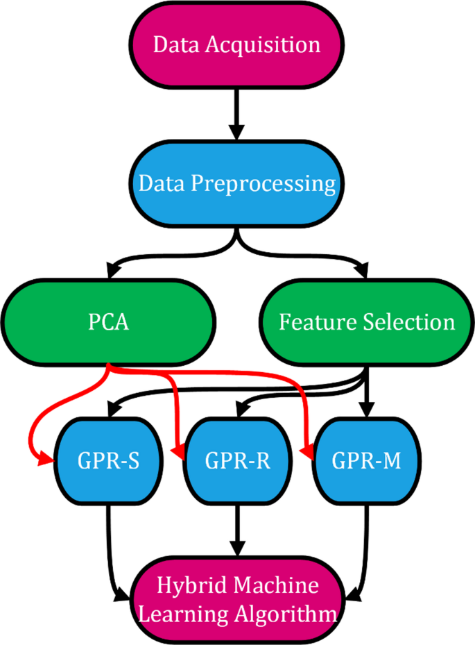
The study was conducted in accordance with the flowchart presented in Fig. 1. In the first step, data acquisition included anthropometric measurements, demographic information, and outputs obtained from bioelectrical impedance analysis (BIA). Then, data preprocessing was performed, which involved handling missing values, normalization, and removal of outliers. The preprocessed data were directed into two dimensionality reduction/feature selection pathways: Principal Component Analysis (PCA) and Spearman correlation-based feature selection. The resulting feature subsets were subsequently used as inputs for three different Gaussian Process Regression (GPR) models: GPR-S (Squared Exponential kernel), GPR-R (Rational Quadratic kernel), GPR-M (Matern52 kernel). Finally, the outputs of these models were combined under a hybrid machine learning algorithm using an ensemble averaging strategy to obtain the final prediction. Since males and females differ significantly in terms of body composition40, gender-specific models were also developed in this study to improve predictive accuracy and account for physiological variation.
Data collectionParticipants
The study was conducted on volunteers who agreed to participate within the Sakarya University campus. Data collection took place between September 2023 and February 2024. The sample comprised 196 males and 289 females, aged 19 to 64 (Table 1). This study was conducted per the ethical standards of the institutional and/or national research committee and with the 1964 Helsinki Declaration and its later amendments or comparable ethical standards. Ethical approval was obtained from the Erciyes University Faculty of Medicine Clinical Research Ethics Committee (Approval Number: 2023/424, Approval Date: 14.06.2023). Written informed consent was obtained from all individual participants included in the study. Permission for data collection was granted by the Rectorate of Sakarya University (Document No: E-35955870-044-268791, Date: 03.08.2023).
Measurements
Data were collected from individuals through questionnaire forms by face-to-face interview method, and bioelectrical impedance analyses (BIA) were performed. 87 demographic and bioelectrical impedance analysis (BIA)-derived variables were collected for each participant. To improve clarity and transparency, the correspondence between feature numbers and their variable names is provided in Table 2. Mapping of Feature Numbers to Variable Names. This table ensures that the feature numbers presented in the results (e.g., Table 2) can be directly interpreted concerning their physiological or demographic meaning.
The questionnaires included data on participants’ demographic characteristics and physical activity status. Parameters obtained via BIA, such as body weight (kg), lean mass weight (kg), lean mass percentage (%), fat mass (kg), fat percentage (%), body fluid weight (kg), and fluid percentage (%), were used in the analyses (Table 2).
Bioelectrical impedance analysis (BIA) was conducted using the Tanita BC-601 Segmental Body Composition Monitor (Tanita Corporation, Tokyo, Japan). This device employs an 8-electrode segmental measurement system providing whole-body and regional assessments (arms, legs, trunk). It has a maximum weight capacity of 150 kg, with a measurement precision of 100 g for body weight and 0.1% for body fat percentage. The device operates at a frequency of 50 kHz, 500 µA, a low-level current that complies with international safety standards for biological measurements. The BC-601 also allows storage and transfer of results via SD card and proprietary software. Calibration was performed automatically per the manufacturer’s guidelines before each measurement session. The validity and reliability of this model have been confirmed in previous clinical studies, and it is widely used in research settings for body composition analysis.
Energy requirement calculation
Energy requirements were calculated based on age, height, and gender using the formula established by the World Health Organization (WHO) (Eqs. 1 and 2). In this formula, the constant value is accepted as 1 for males (Eqs. 1) and 0.95 for females (Eq. 2)41. The authors do not select these constants, but are predefined in the WHO guidelines to account for metabolic differences between males and females. Physical activity level (PAL) is a fixed coefficient that ranges between 1 and 2.5 depending on the daily activity level of the individual, and is incorporated into the Eqs7,41. PAL values of 1–1.39 are used for sedentary activity levels, 1.4–1.59 for light activity, 1.6–1.89 for moderate activity, and 1.9–2.5 for high physical activity levels, respectively41.
$${\text{BMR }}\left( {{\text{male}}} \right){\text{: body weight }}\left( {{\text{kg}}} \right){\text{x constant }}\left( {{\text{1 kcal/kg}}} \right){\text{ x 24}}$$
(1)
$${\text{BMR }}\left( {{\text{female}}} \right){\text{: body weight }}\left( {{\text{kg}}} \right){\text{x constant }}\left( {{\text{0,95 kcal/kg}}} \right){\text{ x 24}}$$
(2)
Spearman feature selection algorithm
Table 3 presents the number of selected features by gender at different percentage levels using the Spearman feature selection algorithm. The selected features are grouped progressively as 5%, 10%, 15%, and so on, up to 100%. Each level represents a specific proportion of the total features selected, and these selections are made to reduce model complexity and optimize performance. The table provides a comparative overview of the number of features selected for males (M), females (F) and total (T). The findings indicate that the number of selected features at each level is similar, mainly between males and females. This suggests that similar features may be equally crucial for model performance in both genders. Notably, at higher levels (80–100%), a more significant number of features were selected for all individuals, indicating that the model operates at its highest level of complexity and utilizes all available features. These results demonstrate that the AI-based model may produce more accurate and reliable estimates of energy requirements by accounting for gender-specific differences. In this study, the term level refers explicitly to the feature subsets generated by the Spearman method. Each level corresponds to a different combination of the original input variables, starting from the most strongly correlated feature (Level 1) to the complete feature set (Level 20). Levels do not introduce new models, weights, or data; they define which subset of features is used for model training.
Machine learning
This study’s most successful machine learning models included Gaussian process regression (GPR) with squared-exponential, rational-quadratic, and Matern52 kernels and a hybrid algorithm.
GPR model
Gaussian process regression (GPR) models are flexible, robust, and non-parametric. They are preferred in high-dimensional, small-sample, or non-linear datasets42. GPR works by learning non-linear mappings through kernel functions, constructing a covariance matrix between input features and real-valued outputs. In this way, it provides Gaussian uncertainty estimates for predictions, which enables integration into predictive control, adaptive control, and Bayesian filtering techniques43.
GPR is simpler compared to neural networks and support vector machines. It possesses non-parametric flexibility and may self-adjust its hyperparameters43. However, some recent approaches—such as the variance-adjusted gradient boosting algorithm—have enhanced the performance of GPR, making it comparable to or even superior to other regression methods like random forests and gradient boosting machines42.
GPR models are commonly used to fit data when the regression function is unknown44. For instance, they are widely utilized in system modeling, forecasting, control techniques, and industrial processes43,45,46. Additionally, GPR has been applied in diverse areas as estimating unknown functions, modeling and forecasting human mortality rates, and predicting the safety margin of a nuclear power plant46.
GPR models may not be effectively used with large datasets due to their high computational complexity. They scale cubically with the number of observations, restricting their use to small- and medium-sized datasets. Consequently, GPR models are powerful tools for probabilistic regression however, their applicability to large-scale data remains limited47.
GPR squared exponential (GPRS), GPR rational quadratic (GPRR), and GPR matern52 (GPRM) are different kernel functions used within the GPR framework. Each function has distinct characteristics that influence the behavior and performance of the GPR model.
To enhance model performance, hyperparameters of the Gaussian Process Regression (GPR) models (e.g., kernel length-scale and variance) were optimized using automated search strategies. These strategies included Bayesian optimization and randomized/grid search techniques, which iteratively adjust parameter values to minimize prediction error based on log-marginal likelihood. This process ensured that the selected kernel configurations provided the best trade-off between model accuracy and generalizability.
GPR squared exponential
GPR squared exponential (GPRS), also known as the Radial Basis Function (RBF), operates assuming the modeled function is smooth and continuous. Its flexibility and smoothness contribute to its frequent use. It is an effective method for capturing complex data relationships48.
GPR rational quadratic
It is a mixture of GPRS functions with different length scales. Compared to GPRS, it is more flexible and capable of producing models with varying degrees of smoothness3. This kernel is particularly used when the data exhibit different levels of variability45.
GPR matern52
It is smoother than the GPRS kernel. However, it behaves more flexibly when constructing rougher models. It provides a good balance between flexibility and smoothness. It is frequently preferred in cases where the underlying function is less smooth47.
Hybrid machine learning algorithm
It is a combination of different algorithms aimed at solving complex problems. By integrating the advantages of multiple algorithms, it seeks to create a more powerful solution method49,50. There are two distinct types of hybridization: collaborative and integrative. Collaborative hybridization approaches the problem by applying the algorithms sequentially or in parallel, allowing for information exchange. Integrative hybridization, on the other hand, focuses on different aspects of the problem-solving process for each algorithm51.
Hybrid algorithms enable more efficient and effective outcomes by combining various techniques. They improve exploration strategies and enhance solution quality52. They exhibit better performance than conventional algorithms, particularly in solving non-deterministic polynomial-time challenging optimization problems, thereby generating a synergistic effect53. These algorithms have been successfully applied to real-world problems52,53. In summary, hybrid algorithms combine the strengths of different approaches to offer more balanced and practical solutions, leading to successful implementations.
In the present study, the hybrid approach integrates three Gaussian Process Regression (GPR) models with different kernels (squared exponential, rational quadratic, and Matern52). Each model was trained independently, and their prediction outputs were combined by taking the simple arithmetic mean (unweighted average) to obtain the final estimate. No specific weights were applied to individual models. This averaging strategy corresponds to a collaborative hybridization, as parallel models contribute to a consensus result. The rationale for this design is that each kernel captures different structural characteristics of the data, and combining them reduces variance, balances individual weaknesses, and improves the overall robustness of the predictions.
Performance evaluation criterion
In machine learning models, performance evaluation criteria (PEC) are essential for selecting the appropriate model for a given task. Depending on the characteristics of the model and user expectations, various experiments may be designed to assess performance. Techniques such as cross-validation and bootstrapping may be used for performance evaluation in supervised and unsupervised models54. In addition, metrics like accuracy, precision, recall, F1 score, and area under the ROC curve are key indicators for assessing model performance55. In supervised learning, models are trained with input data and target variables. In unsupervised learning, only input data is used, and the algorithm attempts to identify patterns within the data56. In the current study, to evaluate the results, the following metrics were employed: Mean Absolute Percentage Error (MAPE), Mean Absolute Deviation (MAD), Standard Error (SE), Mean Squared Error (MSE), Root Mean Squared Error (RMSE), R, and R² (Eqs. 1–5).
MAPE provides a mapping procedure based on measurable criteria and allows for a visual presentation of the results57. It is used in research and development organizations to evaluate performance against specified targets58,59. MAPE is calculated by averaging the absolute percentage errors between predicted and actual values. It is a simple and easily interpretable method; however, it is sensitive to outliers and unsuitable for cases where exact values are zero or near zero60.
MAD is a method that estimates dispersion for continuous and finite-valued random variables without relying on absolute values61. It is especially appropriate when data are skewed and is easy to apply and interpret62.
MSE measures the average of the squared errors or deviations and provides detailed insights into model performance63,64,65. SE measures the accuracy of predictions and indicates the precision of the estimates66.
R² shows the proportion of variance in the dependent variable that the independent variables can explain. However, when used alone as a PEC, it may be insufficient, as it does not indicate which aspects of model performance are strong or weak67,68,69. Among the PECs used in this study, values of MAPE, MAD, SE, MSE, and RMSE are expected to be close to 0, while R and R² are expected to be close to 1.
In addition to the classical error-based metrics (MAPE, MAD, SE, MSE, RMSE, R, and R²), computational efficiency indicators were also considered: Prediction Speed (PS) expressed as observations predicted per second, Training Time (TT) measured in seconds required for model training, and Model Size (MS) measured in kilobytes. These parameters provide practical insights into the computational cost and feasibility of the models, which are critical for clinical and field applications.
In the equations, n represents the total number of data points, t denotes the actual value for each individual, and y denotes the calculated value.
$$MAPE=\frac{1}{n}\sum\limits_{{i=1}}^{n} {\frac{{|{t_i} – {y_i}|}}{{{t_i}}}} \times 100$$
(1)
$$MAD=\frac{1}{n}\sum\limits_{{i=1}}^{n} {|{t_i} – {y_i}|}$$
(2)
$$SH=\sqrt {\frac{{\sum\limits_{{i=1}}^{n} {{{({t_i} – {y_i})}^2}} }}{{n – 2}}} =\sqrt {\frac{{\sum\limits_{{i=1}}^{n} {{e_i}^{2}} }}{{n – 2}}}$$
(3)
$$MSE=\frac{1}{n}\sum\limits_{{i=1}}^{n} {{e_i}^{2}}$$
(4)
$$RMSE=\sqrt {\frac{1}{n}\sum\limits_{{i=1}}^{n} {{e_i}^{2}} }$$
(5)
For testing model performance, the dataset was split into 80% for training and 20% for testing. The training set was used to enable the models to learn, while the test set was reserved to measure the generalizability of performance. During the modeling process, different algorithms were applied, and gender-based models were utilized to enhance performance. Feature selection techniques were employed to achieve higher accuracy with fewer but more effective inputs.
Model variations
Various combinations of gender, feature groups, and AI models were used to develop a total of 240 predictive models in this study. Table 4 summarizes how these model variations were structured. It shows the distribution of 3 gender categories (male, female, and total), 20 different feature groups (see Table 3), and 4 AI model types (GPR-M, GPR-R, GPR-S, and a hybrid model). The resulting combinations outline the whole architecture of the modeling strategy. 240 models (3 genders × 20 feature levels × 4 AI models) were structured to represent different input–algorithm configurations.
k-fold cross-validation
To ensure the robustness and generalizability of the developed models, k-fold cross-validation was employed. This approach randomly partitioned the dataset into k equally sized folds. At each iteration, one fold was used as the validation set, while the remaining k-1 folds were used for training. This process was repeated k times so that each fold was used once for validation. The final performance metrics were obtained by averaging the results across all folds. This procedure reduces the risk of overfitting and provides a more reliable estimate of model performance, particularly when working with relatively small datasets. This study set k to 10, a commonly used choice in the literature for balancing computational efficiency and statistical reliability.
Principal component analysis (PCA)
Strong correlations among high-dimensional datasets may increase model complexity and reduce predictive accuracy. For this reason, dimensionality reduction methods are frequently employed in AI-based modeling studies to maintain model simplicity while enhancing generalizability. Principal Component Analysis (PCA) is a statistical technique that represents correlated variables with fewer independent components, thereby eliminating redundancies in the data while preserving information content70,71.
This study applied PCA directly to the dataset and subsequently integrated into the AI-based modeling process. PCA was used independently as an alternative dimensionality reduction method, rather than in conjunction with Spearman-based feature selection.
Computational platform
All computational analyses were conducted using MATLAB R2024b (MathWorks Inc., Natick, MA, USA). Standard toolboxes such as the Statistics and Machine Learning Toolbox were utilized where available, while all remaining procedures—including feature selection implementation, hybrid model construction, and performance evaluation—were coded manually by the authors. This ensured flexibility in model development and allowed adaptation of the algorithms to the specific requirements of the study.