
 system in Yellow River Basin, China")
The Yellow River Basin (YRB), one of China’s most strategically important regions, flows through nine provinces, encompassing diverse terrains and playing a pivotal role in national development (Fig. 2). In 2020, 15.14% of China’s total population resided in the YRB, with a high concentration in downstream areas. This population distribution has led to significant demographic pressure, particularly in urban regions where more than half of the cities are resource-based or old industrial cities reliant on mineral extraction and processing26. These activities have driven regional economic growth but also intensified competition for resources and heightened environmental risks.
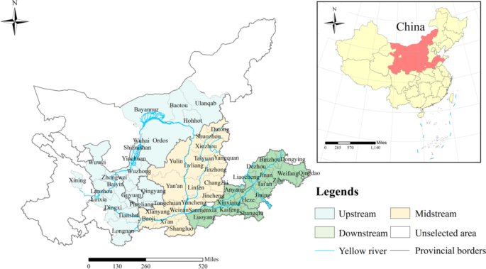
Study area. Source: Created by the authors using ArcMap 10.8 (Esri, Redlands, CA, USA; https://www.esri.com.)
In terms of economic performance, the YRB contributes 20% of China’s GDP, underscoring its importance to national productivity27. However, the basin’s economic development faces structural challenges. Heavy reliance on traditional industries has led to resource over-exploitation, environmental degradation, and inefficiencies in economic growth. Resource shortages, particularly in water and minerals, are becoming critical constraints. Soil erosion and the degradation of cultivated land further weaken agricultural productivity, jeopardizing food security and rural livelihoods28.
Environmental challenges in the basin are deeply intertwined with resource pressures. The region’s fragile ecological systems are vulnerable to overuse and high-intensity human activities, which have caused severe damage. Widespread soil erosion, deforestation, and overgrazing have destabilized ecosystems, while extensive water extraction has contributed to persistent water shortages. Pollution of air, land, and water adds another layer of complexity, severely impacting public health and ecological sustainability29,30.
The combined impact of these pressures—population growth, resource depletion, environmental degradation, and economic constraints—has created a critical need for balance. Historically, development in the YRB has been marked by conflicts between economic expansion and environmental protection, particularly as high-intensity human activities have strained the basin’s resources and ecosystems31,32. Achieving sustainable development in the basin requires reconciling these conflicts through coordinated efforts to harmonize population growth, resource management, environmental restoration, and economic restructuring.
Research methodsEntropy-Topsis model
The entropy-Topsis model has been widely applied in urban complex systems coordination research33. First, data standardization is required to eliminate differences in data caused by different dimensions.
$$Y_{ij} = \left\{ {\begin{array}{*{20}l} {\frac{{X_{ij} – \min (X_{ij} )}}{{\max (X_{ij} ) – \min (X_{ij} )}}} & {\quad {\text{postive}}\;{\text{indicator}}} \\ {\frac{{\max (X_{ij} ) – X_{ij} }}{{\max (X_{ij} ) – \min (X_{ij)} }}} & {\quad {\text{negative}}\;{\text{indicator}}} \\ \end{array} } \right.$$
(1)
where, i represents the city i in YRB, j represents the indicator of the index system, \(X_{ij}\) is the initial value, and \(Y_{ij}\) represents the normalization result of \(X_{ij}\).
Then, the entropy value \(E_{j}\) and indicator weight \(W_{ij}\) would be calculated to build the weighted normalized decision matrix. And the weighted matrix R of the PREE index system is constructed.
$$E_{j} = \ln \frac{1}{n}\sum\limits_{i = 1}^{n} {\left[ {\left( {Y_{ij} /\sum\limits_{i = 1}^{n} {Y_{ij} } } \right)\ln \left( {Y_{ij} /\sum\limits_{i = 1}^{n} {Y_{ij} } } \right)} \right]}$$
(2)
$$W_{ij} = (1 – E_{j} )/\sum\limits_{j = 1}^{m} {(1 – E_{j} )}$$
(3)
$$R = (r_{ij} )_{n \times m}$$
(4)
where, \(r_{ij}\) should satisfy \(r_{ij} = W_{j} \times Y_{ij}\).
Next, according to the weighted matrix R, the optimal scheme \(Q_{j}^{ + }\) and the worst scheme \(Q_{j}^{ – }\) are determined. Calculate the Euclidean distance between each measurement scheme \(d_{i}^{ + }\) and the optimal and worst schemes \(d_{i}^{ – }\).
$$\begin{gathered} Q_{j}^{ + } = (\max r_{i1} ,\;\max r_{i2} ,\; \ldots ,\;\max r_{im} ) \hfill \\ Q_{j}^{ – } = (\min r_{i1} ,\;\min r_{i2} ,\; \ldots ,\;\min r_{im} ) \hfill \\ \end{gathered}$$
(5)
$$\begin{gathered} d_{i}^{ + } = \sqrt {\sum\limits_{j = 1}^{m} {(Q_{j}^{ + } – r_{ij} )^{2} } } \hfill \\ d_{i}^{ – } = \sqrt {\sum\limits_{j = 1}^{m} {(Q_{j}^{ – } – r_{ij} )^{2} } } \hfill \\ \end{gathered}$$
(6)
Last, calculate the relative proximity \(C_{{_{i} }}\) of each measurement scheme to the ideal scheme. \(C_{i}\) ranges from 0 to 1.
$$C_{i} = \frac{{d_{i}^{ – } }}{{d_{i}^{ + } + d_{i}^{ – } }}$$
(7)
Coupling coordination degree model
The coupling coordination degree is frequently used to assess the balance and interaction within urban complex systems comprising multiple subsystems, aiding in the evaluation of urban sustainability19,34.
$$C = \frac{{\sqrt[4]{{P \times R \times E_{1} \times E_{2} }}}}{{{{\left( {P + R + E_{1} + E_{2} } \right)} \mathord{\left/ {\vphantom {{\left( {P + R + E_{1} + E_{2} } \right)} 4}} \right. \kern-0pt} 4}}}$$
(8)
where, C represents coupling degree of PREE system, and \(P\) represents population subsystem, \(R\) represents resource subsystem, \(E_{1}\) represents environment subsystem, \(E_{2}\) represents economy subsystem.
$$T = \alpha P + \beta R + \gamma E_{1} + \mu E_{2}$$
(9)
$$D = \sqrt {C \times T}$$
(10)
T is the integrated index of PREE systems. Four subsystems are equally important in this research, so the coefficients of each subsystem would be set as \(\alpha = \beta = \gamma = \mu = 1/4\). D is the coupling coordination degree of PREE system. The coupling coordination degree is classified into ten levels25, extreme dysfunctional decline (0 ≤ D < 0.1), serious dysfunctional decline (0.1 ≤ D < 0.2), moderate dysfunctional decline (0.2 ≤ D < 0.3), mild dysfunctional decline (0.3 ≤ D < 0.4), on the verge of dysfunctional decline (0.4 ≤ D < 0.5), barely coupling coordination (0.5 ≤ D < 0.6), primary coupling coordination (0.6 ≤ D < 0.7), moderate coupling coordination (0.7 ≤ D < 0.8), good coupling coordination (0.8 ≤ D < 0.9), quality coupling coordination (0.9 ≤ D < 1.0).
Spatial autocorrelation
Moran’s I index is often used to measure the degree to which an area is related to its neighbors. To explore the spatial correlation of the synergistic development of PREE, global autocorrelation was carried out to measure the CCD16.
$$Moran\text{‘}s \, \;I = \frac{{n\sum\nolimits_{i = 1}^{n} {\sum\nolimits_{j = 1}^{n} {W_{ij} (x_{i} – \overline{x} )(x_{j} – \overline{x} )} } }}{{\sum\nolimits_{i = 1}^{n} {\sum\nolimits_{ = 1}^{n} {W_{ij} \sum\nolimits_{i = 1}^{n} {(x_{i} – \overline{x} )^{2} } } } }}$$
(11)
where, \(W_{ij}\) is the spatial adjacency matrix, \(x_{i}\) represents the CCD results of city i, \(\overline{x}\) is the average value of the CCD results in the basin, n is the amount of the YRB cities.
The objective of local spatial autocorrelation is to provide a perspective on how regional differences in spatial processes impact the overall spatial pattern by focusing on variances in small-scale spatial processes. Compared with global spatial autocorrelation, it can more accurately reflect the local characteristics and spatial heterogeneity10.
$$G_{i}^{*} (d) = \frac{{\sum\nolimits_{j = 1}^{n} {W_{ij} (d)x_{j} } }}{{\sum\nolimits_{i = 1}^{n} {X_{i} } }}$$
(12)
$$Z(G_{i}^{*} ) = \frac{{G_{i}^{*} – E(G_{i}^{*} )}}{{\sqrt {Var(G_{i}^{*} )} }}$$
(13)
where \(G_{i}^{*}\) represents the statistic of Getis-Ord, d represents the distance. \(E(G_{i}^{*} )\) is the mathematic expectation of \(G_{i}^{*}\), and \(Var(G_{i}^{*} )\) represents the deviation.
Kernel density estimation
Kernel density estimation is a key non-parametric method that does not rely on assumptions about data distribution. It generates a continuous probability density curve based on the data’s inherent distribution characteristics, enabling a visual representation of the variables’ temporal evolution trend35.
$$f(x) = \frac{1}{nh}\sum\limits_{i = 1}^{n} {K\left( {\frac{{\overline{x} – X_{i} }}{h}} \right)}$$
(14)
where \(K\left( {\frac{{x – X_{i} }}{h}} \right)\) represents the kernel function, \(X_{i}\) is the CCD results of PREE system, \(\overline{x}\) is the mean value, n represents the amount of YRB cities.
GeoDetector model
The geodetector model aims to detect the consistency of the spatial stratified heterogeneity between the dependent variable and independent variables and measures the explanation degree and the interactions between independent variables36. The factor detection and interaction detection models will be used to explore the impact, as confirmed by previous studies37,38. In the factor detection model, q is the key value to evaluate the explanation degree of independent variables to dependent variable.
$$\begin{gathered} q = 1 – \frac{{\sum\nolimits_{h = 1}^{L} {N_{h} \sigma_{h}^{2} } }}{{N\sigma^{2} }} = 1 – \frac{SSW}{{SST}} \hfill \\ SSW = \sum\nolimits_{h = 1}^{L} {N_{h} \sigma_{h}^{2} } ,\;\;SST = N\sigma^{2} \hfill \\ \end{gathered}$$
(15)
where h = 1, L represents the strata of the dependent variable Y or independent variable X. \(N_{h}\) and \(N\) represent the units of strata h and research area. SSW represents the Within Sum of Squares, and SST represents the Total Sum of Squares.
The interaction detection model is set to identify the interaction among the independent variables. Specifically, it aims to evaluate whether the combination of independent variables X1 and X2 would increase or decrease the explanation power, or whether the impacts of these factors on Y are independent.
Indicator selectionIndex construction
The Population-Resource-Environment-Economy (PREE) index system was developed following scientific, systematic, and comprehensive guidelines to ensure a holistic evaluation of regional sustainable development (Table 1). The selection of indicators was carefully considered to reflect the multidimensional aspects of each subsystem.
For the population subsystem, indicators were selected based on the scale-structure-quality framework39. The total population and natural growth rate were included to assess overall population size and growth dynamics, reflecting demographic trends25. The urbanization rate was chosen to represent the structural shift from rural to urban areas, providing insight into urban development and population distribution40. Hospital and educational infrastructure were selected as indicators of living standards because they directly impact the quality of life and social well-being18. These indicators represent the core dimensions of population development, ensuring a balanced assessment of demographic size, structure, and quality.
In the resource subsystem, indicators were chosen to capture resource attributes, structure, and utilization efficiency. Per capita water and arable land reflect the availability of essential resources for human and agricultural use, which are critical for sustainability17. The proportion of agriculture in water and land use was included to reflect resource structure, indicating the extent of land and water resources dedicated to agricultural production41. For utilization efficiency, water and energy consumption relative to GDP were selected to measure how effectively resources are being utilized in economic activities42. These indicators provide a comprehensive view of resource availability, structural use, and efficiency.
The environmental subsystem indicators were based on the Pressure-State-Response (PSR) framework19,43, assessing environmental pressures, conditions, and responses. The pressure dimension includes indicators for major pollution sources, such as carbon dioxide emissions, PM2.5 levels, and industrial sulfur dioxide emissions, reflecting the environmental burden from human activities24. The state dimension measures overall environmental conditions through indicators like NDVI (Normalized Difference Vegetation Index) and park green space area per capita, reflecting urban greenery and ecosystem health25. In the response dimension, the green coverage rate of built-up areas and the proportion of days with good air quality were selected. The latter was chosen to reflect the effectiveness of air quality management and the success of measures taken to improve environmental quality, as more days of good air quality indicate better environmental governance and successful mitigation of pollution42. This indicator was placed in the response dimension because it directly measures the outcome of efforts to improve air quality and environmental health.
For the economy subsystem, indicators followed the scale-structure-quality framework. GDP and fixed asset investment were selected to assess the economic scale, providing insight into overall economic size and infrastructure investments44. The proportion of second and tertiary industries was chosen to represent the economic structure, highlighting the shift from primary industries (e.g., agriculture, mining) to secondary and tertiary industries (e.g., manufacturing, services) that contribute to higher economic value and sustainability24. Finally, the annual GDP growth rate and urban per capita disposable income were selected to evaluate economic quality, reflecting dynamic economic performance and residents’ standard of living34.
Driving factors selection
To explore the influencing factors of CCD in YRB, this study chose seven driving factors to identify the driving mechanism (Table 2). GDP per capita (X1) represents the economic development quality. It encompassed not only the pace and scale of economic growth but also the sustainability of economic growth, the improvement of social welfare, the preservation of the environment, and the rationality of economic structure10. The impact of population density (X2) on CCD was reflected in the tension of resource allocation and the pressure on the ecological environment. While high population density is likely to bring dynamism to the urban economy and benefit economic growth40. Industrial advancement (X3) can improve economic output and efficiency, realize the sustainable use of resources, improve the urban ecological environment, and promote the optimization of urban population structure45. With clean technology, green innovation (X4) could foster sustainable economic growth, population growth, resource efficiency, environmental protection, and population quality46. Moreover, the development of openness (X5) could attract more population agglomeration, encourage the process of urbanization, support the coordinated development of resources and economy, promote the improvement and preservation of the environment, and promote the transformation and upgrading of the economy47. The degree of environmental regulation (X6) can help direct employment and population movement, improve resource allocation, and find a balance between environmental preservation and economic growth48. The governance degree (X7) will support the government’s efforts to better regulate and control the macroeconomic environment, guide resource flow toward environmentally friendly and efficient areas, and ultimately aid in maximizing the efficiency of the economy.
Data sources
This research was conducted in 60 cities from 2011 to 2021 in the YRB. Related statistical data was acquired from the China Urban Statistical Book and China Urban and Rural Construction Statistical Yearbook. Water resource data was collected from the Water Resource Bulletin in each province. NDVI data was acquired from MOD13A3 datasets published by NASA on a regular basis. PM2.5 data was collected from the Atmospheric Composition Analysis Group of Washington University in St. Louis. The green innovation data was collected from the patent search and analysis database of the China National Intellectual Property Administration. Missing data were filled by interpolation.