

Since this dataset is essential for predictive analysis and the development of prediction models, the technical validation involves building machine learning models using the data from the records to assess their suitability. The dataset features extensive, cross-sectional solar energy production data directly linked to solar irradiation, weather parameters, and specific household load requirements. Combining these features enables multifaceted analysis, fostering advancements in renewable energy forecasting, climate-sensitive environments, grid management, and energy policy formulation. This dataset aims to aid in designing new energy systems that enhance sustainable energy strategies, demonstrating their potential to accelerate the transition towards renewable energy and carbon neutrality.
As explained in the Data Records Section, the SHEERM dataset includes two sets of data for household consumption data (Load): raw and processed data. The processed set of data has no missing data or outliers. In this technical validation, we will use the processed set of data. Regarding household energy consumption, we ensure no data is missing or outliers through the data acquisition protocol and the data processing done on the server when a data sample is received. Concerning weather data, since the initial data was fetched from the NSRBD, we have checked, and there is no missing data. Regarding the new features added to the NSRBD, they were computed for all entries in the dataset, resulting in no missing data. Regarding photovoltaic energy generation data, since it was computed through Equations (1), (2) and (3), there is also no missing data associated with it.
However, suppose more data is added to the SHEERM dataset, and gaps are generated. In that case, techniques such as those used in our acquisition procedure can be used to fill those gaps. For instance, using an LSTM, the time series data can be predicted for several instances ahead. So, if there is missing data, it can filled with the predicted values generated by the LSTM. Other approaches or statistical models can also be used, such as forward or backward fill, linear interpolation, interpolation with splines or polynomial methods, moving averages, seasonal decomposition, and other machine learning techniques.
The simplest way to fill data gaps may be to use the forward or backward fill, where missing values are filled with the last known value (forward fill) or the next known value (backward fill). This technique is appropriate when consecutive data points, such as short-term missing data, are expected to be similar.
Linear interpolation techniques50 can be used to estimate missing values by connecting the points before and after the gap with a straight line. This technique is suitable for small gaps in data where the values are expected to change linearly. Interpolation with splines or polynomial methods51,52 is another option to fill the gaps. These techniques use polynomial or spline curves to fit the data points and use it to estimate missing values. They are useful when the data has a non-linear pattern.
Moving average techniques53,54,55 can also fill missing values with the average of neighboring data points over a specified window. It is useful when the missing data is part of a more significant trend and smoothing is desired.
A more complex approach can also be used, like seasonal decomposition, where the time series is decomposed into trends (seasonality). Missing values can be filled by estimating from trend behavior. This method is effective when the data has strong seasonal patterns, like weather data. Lastly, similar to what we did in our acquisition procedure, algorithms like K-Nearest Neighbors (KNN), Random Forest, or even deep learning models can be used to estimate missing values53,56,57,– 58. These methods are appropriate for datasets where simple methods might not capture underlying patterns. They are suitable for situations where certain weather events are known, and no statistical model can account for them.
The technical validation aims to verify that our dataset is appropriate for predicting future values for household energy consumption, weather conditions, photovoltaic energy production, and energy market price. Similar to the most relevant datasets presented in the literature (Table 1), for the technical validation, we developed various machine learning methods to conduct several analyses and demonstrate the consistency, accuracy, and usability of the provided data. These include predicting household energy needs, forecasting weather conditions, estimating photovoltaic energy production based on predicted weather conditions, and projecting trends in energy prices. These examples showcase the practical applications of the dataset and the potential insights it can provide.
The machine learning models were implemented using the Python programming language (version 3.11.6), which is supported by several Python libraries. Pandas (version 2.1.1) was employed for data manipulation and analysis, while NumPy (version 1.24.4) helped us with efficient numerical computations. The Matplotlib Python library (version 3.8.0) was also used, aiding us in creating plots for visualizing data trends and patterns. Scikit-learn (version 1.3.1) and TensorFlow (version 2.14.0) were used to implement machine and deep learning models and evaluate their performance metrics. The statsmodels library, version 0.14.0, was also used to perform the linearity analysis.
Household Consumption Data (Load)
The analysis of the household consumption data involves a linearity analysis to assess the underlying data characteristics. Then, we demonstrate the effectiveness of various machine learning models in capturing trends and accurately forecasting household consumption. This approach allows us to assess whether models can provide reliable predictions based on the data’s inherent patterns.
Linearity analysis is an important method for understanding the data and selecting the best predictive model. Since linear models are more easily interpreted and computationally efficient, linearity analysis can assess whether models like linear regression are appropriate or need more complex models. Additionally, understanding the data’s linearity may help to improve the model’s accuracy and prevent overfitting.
Based on Ramsey’s RESET test59 and the Ordinary Least Squares (OLS)60 regression, we designed two approaches for this analysis: 1) considering the entire dataset, where the linearity analysis is performed at once on the entire time series, and 2) considering sliding windows, where the time series is divided into smaller time frames and the linearity analysis is performed on each window separately. The first approach is simple to implement and reduces complexity. It helps identify the overall data behavior in terms of linearity but may overlook local variations of the data that do not fit the global trend. The second approach analyzes smaller data sections (106433 windows were considered), which detect local linear relationships that might not be visible in the overall dataset. This approach is beneficial in the Load data analysis since it is a time series with varying conditions, like day/night, week/weekend, and summer/winter.
Table 9 summarizes the results of our linearity analysis on household consumption data considering different sliding window sizes and the entire time series. The results show the ratio of analyzed windows whose p‐value < 0.05. The study suggests that the data exhibits mostly linear patterns for small window sizes. Ramsey’s RESET test shows that we can not reject the null hypothesis (i.e., the data could be modeled by a linear expression since there is no evidence to suggest that the linear model is misspecified). However, the results suggest that the linear model is misspecified for large window sizes (windows greater than 12 hours), meaning the data follows a non-linear pattern. These results suggest that traditional linear models may not effectively capture the underlying trends. Table 10 This observation highlights the need for machine learning models that are better suited to handle non-linear relationships in predictive modeling.
Regarding machine learning applicability, this technical validation focuses on creating various predictive models using LSTMs, RFR, XGBoost, and MLP algorithms to predict the load values for each house. Since the household data was acquired through certificate equipment (smart meters according to the EC Directive 2004/22/EC), the technical validation of the household data involves creating a predictive model that accurately predicts the load for the houses. We present the architecture of the LSTM model (Table 11) as well as the hyperparameters used for the RFR, XGBoost, and MLP (Table 12), noting that the architecture and the hyperparameters were chosen through applying a grid search optimization algorithm61. The grid search was conducted on the household consumption data, where various intervals of values were evaluated to enhance the model’s performance. The range of values tested for each hyperparameter is represented in Table 10.
The data split was into 75% train and 25% test applied to each household consumption data. Each model, LSTM, XGBost, MLP Regressor, and Random Forest, is trained for each one of the houses (using 75% of the data) and evaluated in the remaining 25%. We compared the real values for the load of the house and the predicted ones. The evaluation metrics used to assess each model include the root mean squared error (RMSE), Mean squared error (MSE), and R-squared (R2). Table 13 presents the evaluation metrics obtained from applying the models to their corresponding test data. All values were forecasted for a timespan of one day ahead (96 points ahead). From the results obtained, we could conclude that, on average, the model that tends to be more accurate according to R2 and leads to fewer errors is the LSTM model.
Based on the R2 results, we identify a good relation between the predicted data and the real data for the LSTM model, meaning that the data can be used to train/develop these machine-learning models and predict the energy needed. Figure 10 graphically represents some of the predicted and real values obtained for the houses for a given day, illustrating the model’s predictive capabilities and, consequently, the validity of the data.
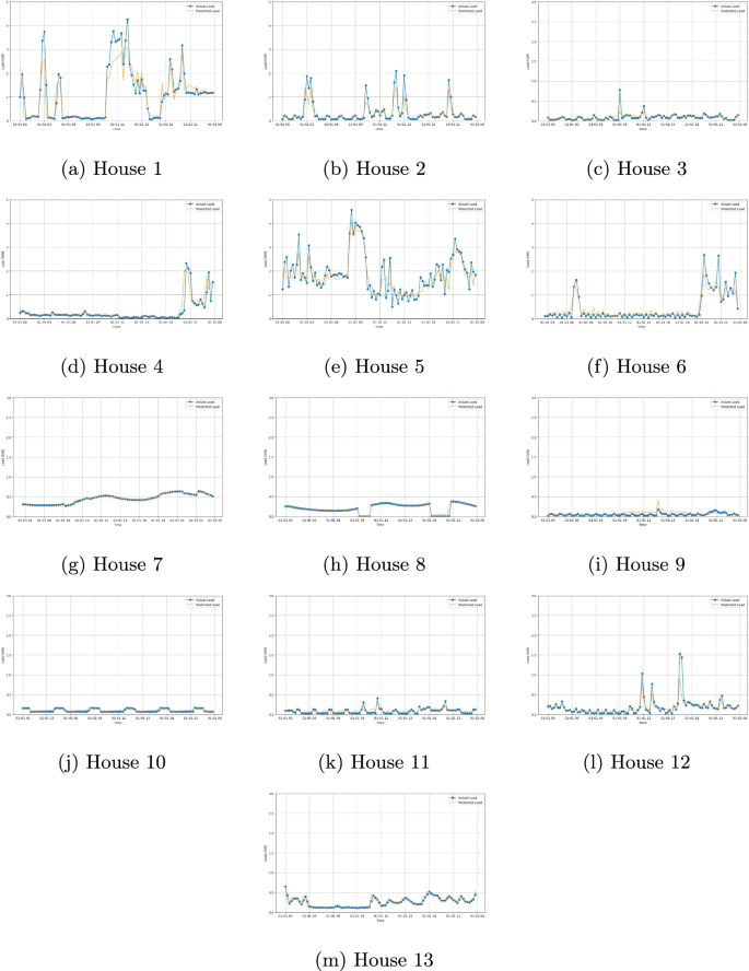
Load predictions for multiple houses using an LSTM model.
Weather and photovoltaic power generation
For the technical validation of weather and photovoltaic power generation prediction, we used two methods. The GHI in SHEERM and a real-world experiment were compared first. Second, LSTM deep learning models are used to predict solar irradiation, and a Random Forest Classifier is used to predict cloud type.
Since the GHI was obtained from an external source (NSRDB), we looked at another dataset to validate the data. Upon an extensive search, we identified the work done by T. Yao62. In this work, the authors provided data for GHI in their location based on a numerical weather prediction (NWP) method63. Since the NSRDB allows us to select any position in the world and fetch data for that position, we identify the locations used by T. Yao’s work and compare the data fetched from NSRDB against their NWP data.
Figure 11 depicts this comparison and shows the similarity between the NSRDB and the NWP data, which allows us to conclude that the data fetched from NSRDB is reliable. However, the data from both sources assume a tilted position of β = 0° of the solar panel, which is only valid for positions on the equatorial line at noon. Since our data was collected in the north hemisphere, a tilt angle is used in the solar panel to maximize the captured energy, which means that the GHI must be corrected to consider this influence. For that, Equation (3) is used. Considering the tilt angle of the panel β = 33°, the estimated GHI is shown through the yellow curve in Fig. 11. As we can see, the panel’s tilt angle significantly influences the quantity of captured solar irradiation. This influence is considered in our data related to the photovoltaic power generation, considering the position of each panel and its configuration.
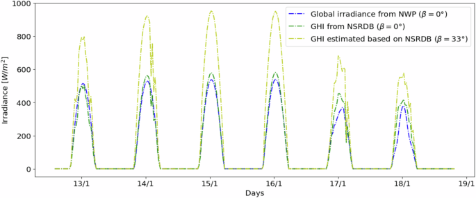
Comparison of the GHI values provided by the NSRDB and NWP considering β = 0°, and the GHI estimated based on the NSRDB considering the tilt angle β = 33° of a location from62.
Tables 14 and 15 represent a summary of the weather data in the dataset per house and region, respectively. Since the outside temperature and humidity influence the efficiency of solar panels, we show these values per house and area, which can help in further analysis, allowing us to adjust the prediction model to reflect real-world conditions according to the region where the houses are.
Moreover, household energy consumption is closely related to temperature variations. Heating and cooling needs fluctuate with temperature changes, making this data vital for accurate consumption forecasting. Precipitation, cloud cover, and wind conditions can also impact solar energy production and household energy use. For instance, cloudy or rainy days might also increase indoor lighting and heating demand.
Regarding photovoltaic power generation data, as detailed in the methodology section, it was computed using Eq. (1)45,46. To assess the reliability of the chosen model and the resulting data contained in the SHEERM dataset, we conducted a comparison between the real-world measurements provided by the Open Power System Data (OPSD) database26 and the corresponding result obtained through Eq. (1). Figure 12 compares the theoretical model results and the real-world measurements. The figure reveals slight deviations between the two, which, upon closer examination, do not appear to stem from inaccuracies in the model itself. Instead, we believe these deviations are likely due to inaccuracies in the solar irradiation measurements from OPSD (i.e., the input data Δ of Eq. (1)). This conclusion is supported by the model consistently following the same trend as the real-world data, often closely matching or overlapping with the measured values. This comparison between the OPSD’s real-world measurements and the results obtained from our theoretical model provides an additional validation step. It allows us to evaluate the reliability of the photovoltaic power generation data included in the SHEERM dataset, ensuring that the theoretical model produces reliable estimations.
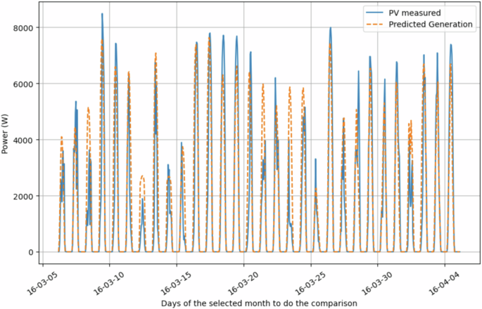
Comparison of Photovoltaic real-world measurements and theoretical model calculations.
We also conducted a linearity analysis on the same data (weather and photovoltaic power generation data). Due to the seasonality inherent in the data, mainly the weather data propagated to the photovoltaic power generation data, the analysis revealed a non-linear trend in both sets of data. For the sake of not being exhaustive, due to the amount of weather and photovoltaic time series, the linearity test values are not incorporated in this article. Still, they can be obtained in our Jupyter notebook (see49).
Since this work aims to contribute to the development of enhanced weather and photovoltaic perdition models, like the one used by R. Peeriga et al.64, Y. Hao et al.65, Z. Hu et al.66 or F. Campos et al.67, for this technical validation, an LSTM is used to demonstrate the usability of the weather dataset. This example involves developing an LSTM to predict the Global Horizontal Irradiance (GHI). Moreover, evaluating a predictive model for GHI values and predicting the Cloud Type is necessary since both can provide deeper insights into the data.
Predicting two main variables, GHI and Cloud Type, are important for determining the solar power generated by a solar panel. Specifically, an LSTM model with the architecture shown in Table 16 was applied to each house to predict GHI, using an 80% training and 20% testing data split. This architecture resulted from a grid search approach, where the range of values tested for each hyperparameter is presented in Table 10.
Regarding cloud type prediction, it is important to accurately determine solar irradiation and, consequently, the solar power generated. Different cloud types have distinct effects on solar irradiation. Some may diffuse or block sunlight more than others, leading to significant variability in the amount of solar irradiation that reaches the solar panel surface. Predicting cloud types allows us to model these variations more precisely, significantly enhancing the accuracy of solar irradiation predictions. This reassures us about the reliability of the data we are working with, making our predictions more robust.
In the context of machine learning, segmenting the problem first to predict cloud types allows us to design more reliable prediction models. This enables us to account for the specific influence of various cloud formations on solar irradiation. For example, high-altitude clouds might partially block sunlight, while dense clouds could significantly reduce solar irradiation. By incorporating this information into our models, we can enhance the predictive performance of solar power generation models, leading to better forecasting systems. Due to its categorical nature, a random forest classifier (RFC) was used to predict the cloud-type variable. The model architecture used comprises n_estimators = 90, max_depth = 22, and random_state = 2024.
From both the LSTM and the RFC models, the evaluation metrics are represented in Table 17. Additionally, Figs. 13 and 14 represent the predicted and real values for both the GHI and Cloud Type. Figure 14 emphasizes the influence of the clouds in the GHI by overlapping both representations. The obtained results show that the predictions for both the GHI and the Cloud Type are good, demonstrating the data’s usability and accuracy.
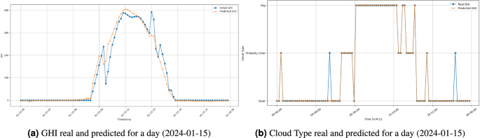
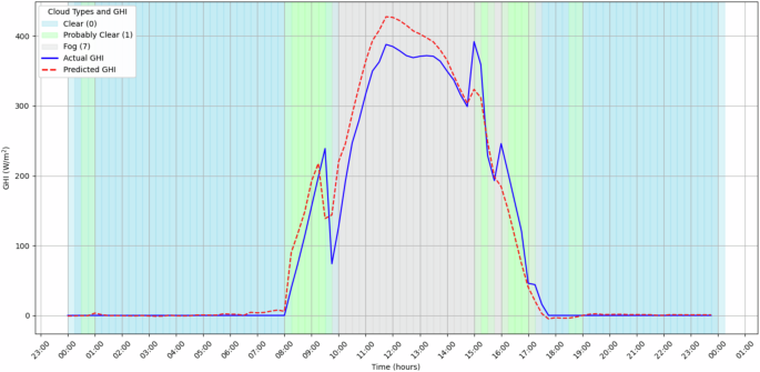
GHI real and predicted with the predicted Cloud Type for a day (2024-01-15).
Market Energy Price Data
In this section, we used the same four machine learning models (LSTMs, RFR, XGBoost, and MLP) to predict household consumption and the gross market price of electricity. The same architecture and hyperparameters for RFR, XGBoost, and the MLP were applied (see Table 12). Concerning the LSTM model, since the energy market price series shows a smoother trend, a new architecture with the configuration represented in Table 18 was applied. Regarding the amount of data used to train and test, the same data portions were used as before (train = 75%, test = 25%).
The Ember-climate dataset provides a comprehensive overview of market prices across the European Union, ensuring that our data is reliable and up-to-date.
The first thing to note is that the prediction is only applied to the values after 2021. Before this date, the values for the price were relatively uniform and did not show any significant changes. However, after 2021, there has been a substantial change in the distribution of values. It is best to apply our model only to that section to better understand the model’s capabilities. To perform this analysis, data from 2021 to 2024 was used for training, and data from the last year was used for prediction.
From the obtained results (Table 19), it is possible to conclude that the model performs better in the LSTM even though all results are very satisfactory. This performance allows us to conclude the SHEERM dataset is reliable and can be used to aid in designing new energy systems that enhance sustainable energy strategies.
Figure 15 compares the actual and predicted energy market prices for a specific day (2023-10-11) forecasted by using the LSTM model. The figure shows a slight deviation between the predicted and real values, with the predictions being slightly lower. This indicates that our predictive model is not fully calibrated and requires further refinement. However, we assume the data is reliable for this validation since the predictions follow the same pattern as the actual values. Moreover, Table 19 shows the values for the evaluation metrics, reinforcing the idea that there are no problems with the data.
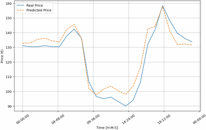
Real and Predicted values for House 1 for a specific day (2023-10-11).
We also analyzed linearity using the market energy price data from the SHEERM dataset. By applying the sliding window approach, we identified windows where linear models may be appropriate, particularly for short-term price forecasting during stable periods. However, the analysis confirms that energy prices are predominantly non-linear, driven by shocks, seasonal patterns, and regulatory interventions. Consequently, non-linear models may be more effective for capturing the dynamics of energy markets. The linearity test values can be obtained through the Jupyter notebook we provide (see49).
Data Correlations
Understanding and analyzing data correlations is fundamental to identifying dataset patterns and dependencies. In the SHEERM context, this analysis allows for an understanding of how variables are correlated with energy consumption behavior. Based on this knowledge, we can enhance the accuracy of predictive models, identify potential causative factors, and inform optimization strategies. This section analyzes the possible correlations presented in the SHEERM dataset. For this analysis, two houses in different regions were selected as case studies. Specifically, houses 1 and 3 were chosen as representative examples.
We first explore the relationship between household energy consumption and external temperature (Fig. 16). This analysis helps determine how much household energy usage is driven by heating or cooling demands, providing insights into how external temperature influences energy consumption behavior.
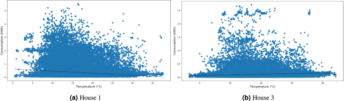
Correlation between household load consumption versus temperature.
As shown in Fig. 16, each house exhibits distinct energy consumption patterns. House 1’s trend indicates that energy consumption tends to increase as temperatures decrease. In contrast, House 3 shows the opposite trend, also with higher energy consumption observed at higher temperatures. These differences can be due to the houses’ locations. They are located in different regions of Portugal, with House 1 in the central coastal zone while House 3 is in the center of Portugal. Typically, in the center of Portugal, heating systems are predominantly fueled by wood, meaning their energy usage is not reflected in household electrical consumption. Contrarily, cooling systems, especially air-conditioning units, rely on electricity, leading to higher energy consumption during warmer temperatures. House 1, located in a region with milder temperature fluctuations and where wood-based heating systems are uncommon, demonstrates a different pattern. Here, household electrical consumption tends to increase during freezing temperatures due to the dependence on electric heating systems.
Regarding the correlation between household energy consumption and energy market prices, Fig. 17 illustrates their relationship and the corresponding trend line. Upon analyzing the trend line, it becomes evident that it has an insignificant slope, indicating that household energy consumption is independent of oscillations in energy market prices for these houses.
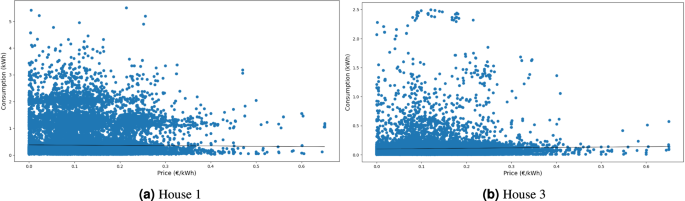
Correlation between household load consumption versus energy market price.
Additionally, we depict the correlation between photovoltaic power generation capacity and solar irradiance. As shown in Equation (1), the power output of solar panels is directly proportional to the irradiance they receive. Figure 18 illustrates this relationship.
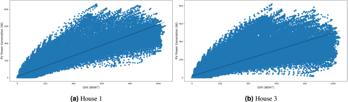
Correlation between photovoltaic energy production and global horizontal irradiance.